Getting Started#

The Chalmers Atmospheric Water Dataset from the Arctic Weather Satellite (AWS), provides global atmospheric ice mass estimates derived from passive microwave measurements. The data are available as NetCDF files, the following examples will show how to get started using them with python and xarray.

[ ]:

from datetime import datetime
import requests
import xarray as xr

# Helper function to get file urls for given timeranges
def file_urls_for_timeranges(timeranges: list[slice]) -> list[str]:
    """
    Get a list of level2 urls for the requested timerange
    """
    base_url = "https://storage.googleapis.com/petermfiles/cawd-aws-v0.0.1-example/level2"
    index = requests.get(f"{base_url}/index.json").json()
    urls = []
    for timerange in timeranges:
        tr_slice = slice(
            datetime.fromisoformat(timerange.start.replace("Z", "+00:00")),
            datetime.fromisoformat(timerange.stop.replace("Z", "+00:00"))
        )
        urls.extend([
            f"{base_url}/{item['filepath']}#mode=bytes"
            for item in index['items']
            if (datetime.fromisoformat(item['datetime_end']) >= tr_slice.start)
            and (datetime.fromisoformat(item['datetime_start']) <= tr_slice.stop)
        ])
    return sorted(set(urls))

[2]:

# List some interesting scenes
timeranges = [
    slice('2025-05-01T07:18:00', '2025-05-01T07:26:00'),
    slice('2025-05-01T11:19:00', '2025-05-01T11:28:00'),
    slice('2025-05-01T11:46:00', '2025-05-01T11:55:00'),
]

# Open the files as a single xarray dataset
ds = xr.open_mfdataset(file_urls_for_timeranges(timeranges))
ds

[2]:

<xarray.Dataset> Size: 117MB
Dimensions:                 (time: 6727, fov: 88, quantile: 5, surface_type: 6,
                             channel: 11)
Coordinates:
  * time                    (time) datetime64[ns] 54kB 2025-05-01T06:05:41.53...
  * surface_type            (surface_type) <U7 168B 'ocean' ... 'glacier'
    latitude                (time, fov) float64 5MB dask.array<chunksize=(3364, 88), meta=np.ndarray>
    longitude               (time, fov) float64 5MB dask.array<chunksize=(3364, 88), meta=np.ndarray>
  * quantile                (quantile) float32 20B 0.01 0.1325 0.5 0.8675 0.99
  * channel                 (channel) <U5 220B 'AWS21' 'AWS31' ... 'AWS44'
Dimensions without coordinates: fov
Data variables: (12/21)
    fwp_mean                (time, fov) float32 2MB dask.array<chunksize=(3364, 88), meta=np.ndarray>
    fwp_most_prob           (time, fov) float32 2MB dask.array<chunksize=(3364, 88), meta=np.ndarray>
    fwp_quantiles           (time, fov, quantile) float32 12MB dask.array<chunksize=(3364, 88, 5), meta=np.ndarray>
    fwp_dm_mean             (time, fov) float32 2MB dask.array<chunksize=(3364, 88), meta=np.ndarray>
    fwp_dm_most_prob        (time, fov) float32 2MB dask.array<chunksize=(3364, 88), meta=np.ndarray>
    fwp_dm_quantiles        (time, fov, quantile) float32 12MB dask.array<chunksize=(3364, 88, 5), meta=np.ndarray>
    ...                      ...
    sim_db_all_ta_distance  (time, fov) float32 2MB dask.array<chunksize=(3364, 88), meta=np.ndarray>
    l1b_index_scans         (time) uint32 27kB dask.array<chunksize=(3364,), meta=np.ndarray>
    l1b_index_fovs          (time, fov) uint32 2MB dask.array<chunksize=(3364, 88), meta=np.ndarray>
    flag_bad_data           (time, fov) uint8 592kB dask.array<chunksize=(3364, 88), meta=np.ndarray>
    flag_overlap            (time) bool 7kB dask.array<chunksize=(3364,), meta=np.ndarray>
    fwp_ccic                (time, fov) float32 2MB dask.array<chunksize=(3364, 88), meta=np.ndarray>
Attributes:
    title:            Chalmers Atmospheric Water Dataset from the Arctic Weat...
    institution:      Chalmers University of Technology
    history:          Retrieval processing
    source_file:      W_NO-KSAT-Tromso,SAT,AWS1-MWR-1B-RAD_C_OHB__20250501074...
    source_file_md5:  d569c33690327feb2f3b925f3172a208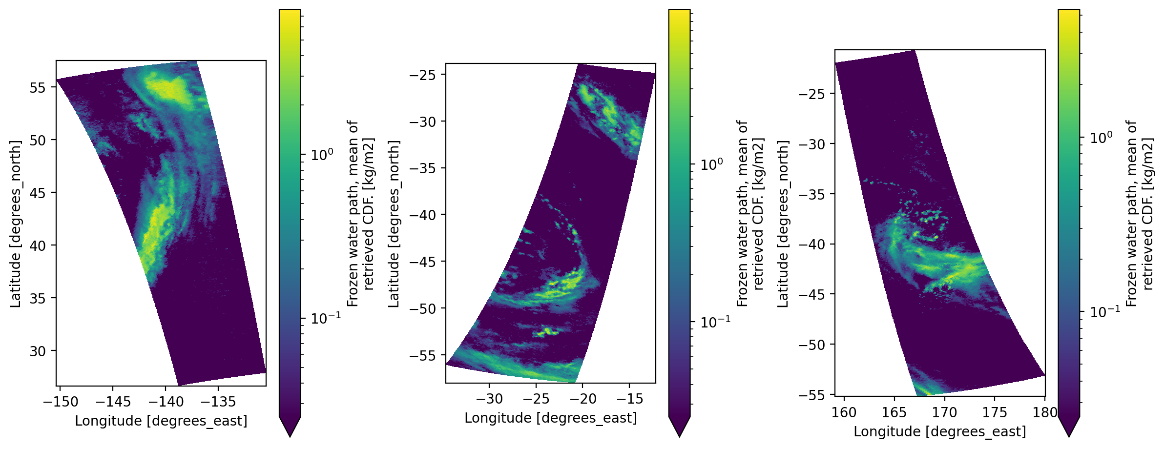
    cache_version:    2b17ed68cfda73625dc987e758a4cd6e9f844d42

Plotting FWP#

[3]:

import matplotlib
import matplotlib.pyplot as plt

# Plot the mean Frozen Water Path (fwp) for our time ranges
fig, axs = plt.subplots(1, 3, figsize=(12, 5), dpi=200, subplot_kw={'aspect': 'equal'})
for ax, timerange in zip(axs, timeranges):
    ds_scene = ds.sel(time=slice(timerange.start, timerange.stop))
    ds_scene.fwp_mean.plot.pcolormesh(
        x='longitude',
        y='latitude',
        norm=matplotlib.colors.LogNorm(vmin=0.025), # Recommended
        ax=ax
    )

plt.tight_layout()

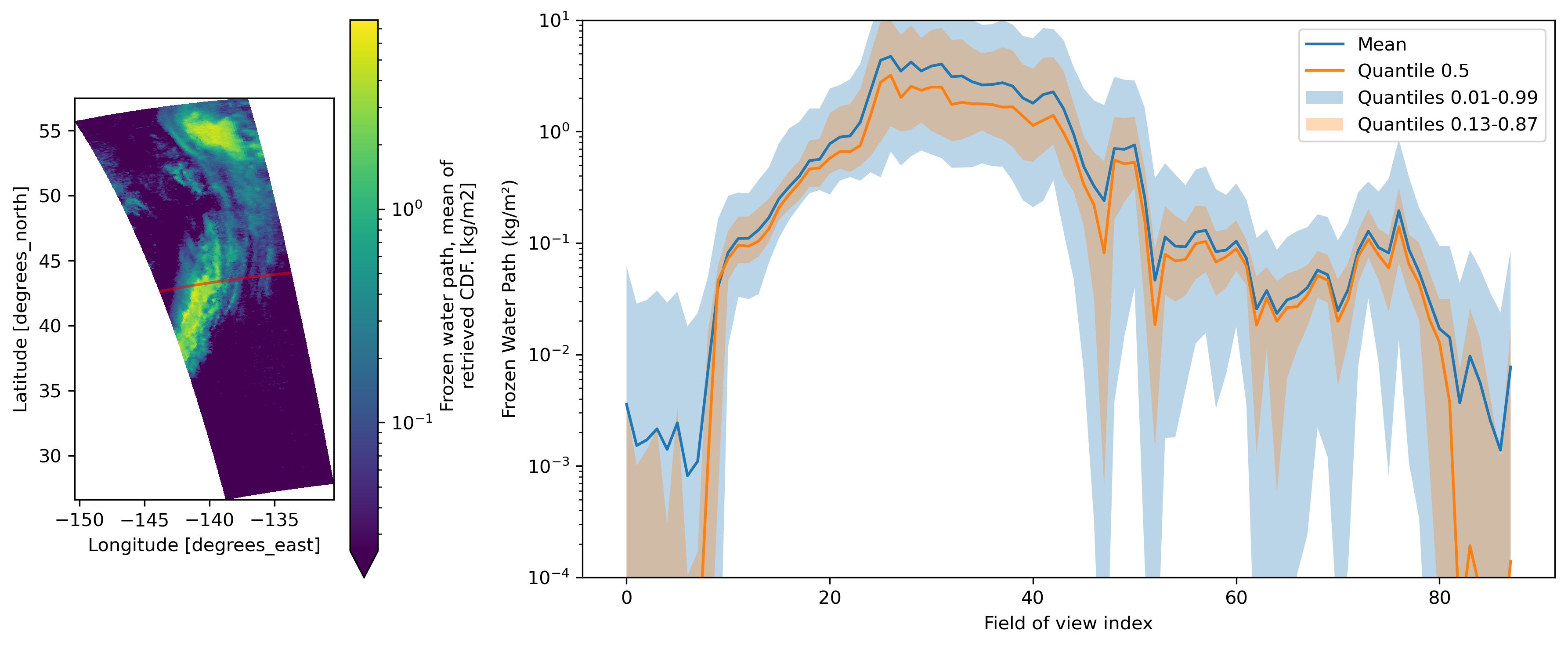
Quantiles#

The retrieval process estimates a cumulative distriubtion function (CDF) for each variable. We’ve so-far been looking at the mean computed from this CDF. Each variable in the dataset also have corresponding quantile values. We can plot these quantiles to get a sense of the estimated distibution of values.

[4]:

fig = plt.figure(figsize=(12, 5), dpi=300)
gs = fig.add_gridspec(1, 2, width_ratios=[1, 3])

# Select a scene and then select a scan within that scene
ds_scene = ds.sel(time=slice(timeranges[0].start, timeranges[0].stop))
ds_scan = ds_scene.isel(time=220)

# Draw map and highlight scan
ax_map = fig.add_subplot(gs[0], aspect='equal')  # Smaller subplot with map projection
ds_scene.fwp_mean.plot.pcolormesh(x='longitude', y='latitude', norm=matplotlib.colors.LogNorm(vmin=0.025), ax=ax_map)
ax_map.plot(ds_scan.longitude, ds_scan.latitude, color='red', alpha=0.5)

# Plot the quantiles for the scan
ax_quantiles = fig.add_subplot(gs[1], xlabel='Field of view index', ylabel='Frozen Water Path (kg/m²)', yscale='log', ylim=(1e-4, 1e1))
ax_quantiles.plot(ds_scan.fwp_mean, label='Mean')
ax_quantiles.plot(ds_scan.fwp_quantiles.sel(quantile=0.5), label='Quantile 0.5')
for i in range(ds_scan['quantile'].size // 2):
    lower = ds_scan.fwp_quantiles.sel(quantile=ds_scan['quantile'][i])
    upper = ds_scan.fwp_quantiles.sel(quantile=ds_scan['quantile'][-(i + 1)])
    ax_quantiles.fill_between(
        x=range(len(lower)),
        y1=lower,
        y2=upper,
        alpha=0.3,
        label=f'Quantiles {ds_scan["quantile"][i].item():.2f}-{ds_scan["quantile"][-(i + 1)].item():.2f}'
    )
ax_quantiles.legend()

plt.tight_layout()

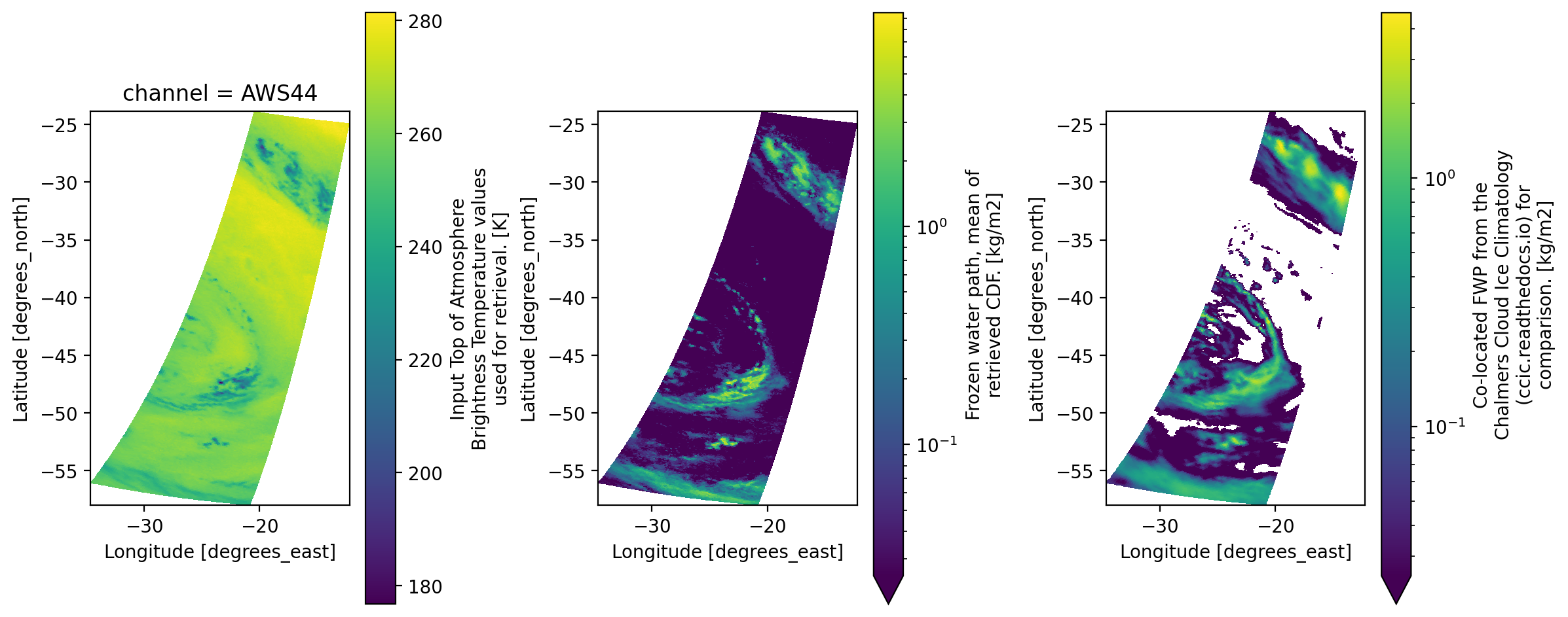
Extra Data#

In addition to retrieved variables, the dataset includes the level1b antenna temperatures remapped to the AWS3X footprint grid and co-located FWP estimates from the Chalmers Cloud Ice Climatology. These can be useful for comparison and for identifying cases based on channel Ta values.

[5]:

fig, axs = plt.subplots(1, 3, figsize=(12, 5), dpi=200, subplot_kw={'aspect': 'equal'})

ds_scene = ds.sel(time=slice('2025-05-01T11:19:00', '2025-05-01T11:28:00'))
ds_scene.tb.sel(channel='AWS44').plot.pcolormesh(x='longitude', y='latitude', ax=axs[0])
ds_scene.fwp_mean.plot.pcolormesh(x='longitude', y='latitude', norm=matplotlib.colors.LogNorm(vmin=0.025), ax=axs[1])
ds_scene.fwp_ccic.plot.pcolormesh(x='longitude', y='latitude', norm=matplotlib.colors.LogNorm(vmin=0.025), ax=axs[2])

plt.tight_layout()

Getting Started#

Plotting FWP#

Quantiles#

Extra Data#

This Page