Interpolating Point Data

Avertissement

This tutorial is now obsolete. A new and updated version is available at Interpolating Point Data (QGIS3)

L’interpolation est une technique courante en SIG pour créer une surface continue à partir d’une série de points. Un grand nombre de phénomènes sont continus dans le monde réel ( l’altitude, le terrain, la température, etc..). Il est impossible de faire des mesures sur l’ensemble de la surface pour les modéliser avant d’en faire l’analyse. C’est pourquoi les mesures sur le terrain sont faites sur plusieurs points répartis sur la surface et les valeurs intermédiaires sont déduites grâce à un traitement appelé l’interpolation. Dans QGIS, l’interpolation est faite en utilisant l’extension native « Interpolation ».

Description de l’exercice

We will take field depth measurements for a Lake Arlington in Texas and create an elevation relief map and contours from these measurements.

Autres compétences que vous allez développer

• Creating contours from point data.

• Masking no-data values from a raster layer.

• Adding labels to a vector layer.

Récupérer les données

Texas Water Development Board provides the shapefiles for completed lake surveys.

Download the 2007-12 survey shapefiles for Lake Arlington.

For convenience, you can directly download the sample data used in this tutorial from link below.

Shapefiles.zip

Data Sources: [TWDB]

Procédure

1. Open QGIS. Go to Layer ‣ Add Layer ‣ Add Vector Layer..

2. Browse to the downloaded Shapefiles.zip file and select it. Click Open.

3. In the Select layers to add… dialog, hold the Shift key and select Arlington_Soundings_2007_stpl83.shp and Boundary2004_550_stpl83.shp layers. Click OK.

4. You will see the 2 layers loaded in QGIS. The Boundary2004_550_stpl83 layer represents the boundary of the lake. Un-check the box next to it in the Table of Contents.

5. This will reveal the data from the second layer Arlington_Soundings_2007_stpl83. Though the data looks like lines, it is a series of points that are very close.

6. Click the Zoom icon and select a small area on the screen. As you zoom closer, you will see the points. Each point represents a reading taken by a Depth Sounder at the location recorded by a DGPS equipment.

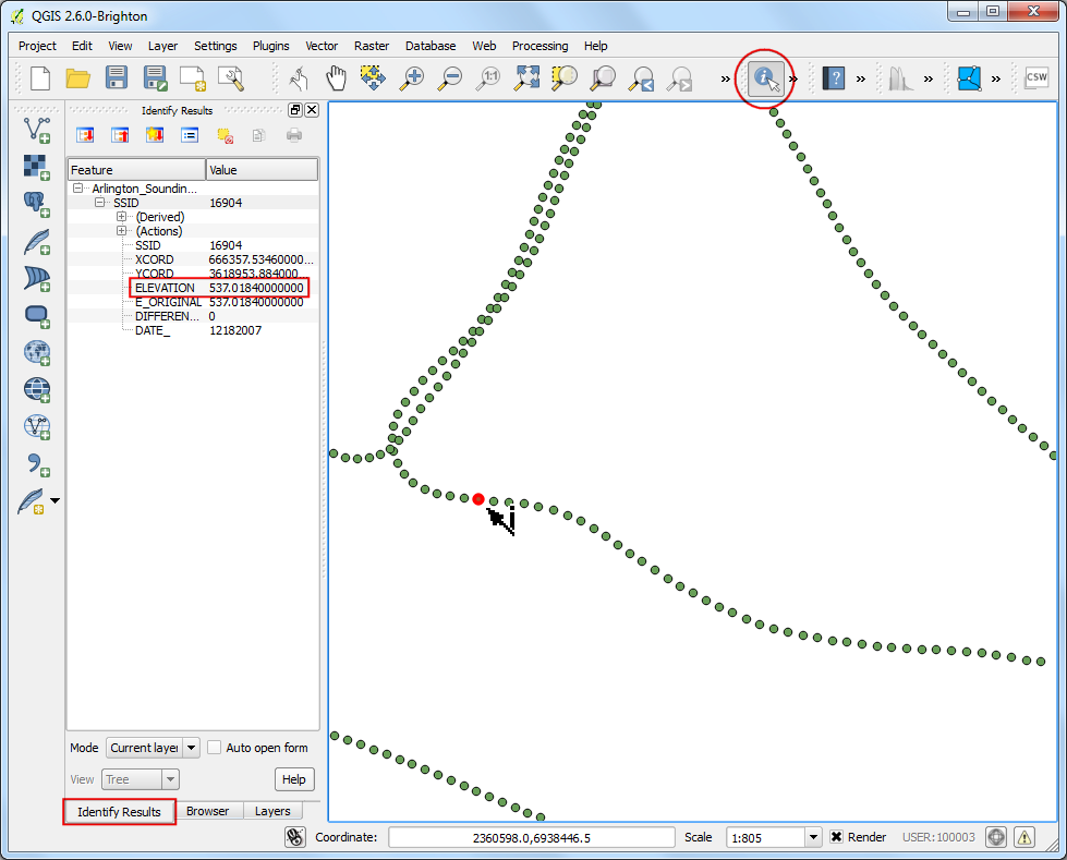
7. Select the Identify tool and click on a point. You will see the Identify Results panel show up on the left with the attribute value of the point. In this case, the ELEVATION attribute contains the depth of the lake at the location. As our task is to create a depth profile and elevation contours, we will use this values as input for the interpolation.

8. Make sure you have the Interpolation plugin enabled. See Using Plugins for how to enable plugins. Once enabled, go to Raster ‣ Interpolation ‣ Interpolation.

9. In the Interpolation dialog, select Arlington_Soundings_2007_stpl83 as the Vector layers in the Input panel. Select ELEVATION as the Interpolation attribute. Click Add. Change the Cellsize X and Cellsize Y values to 5. This value is the size of each pixel in the output grid. Since our source data is in a projected CRS with Feet-US as units, based on our selection, the grid size will be 5 feet. Click on the … button next to Output file and name the output file as elevation_tin.tif. CLick OK.

Note

Interpolation results can vary significantly based on the method and parameters you choose. QGIS interpolation supports Triagulated Irregular Network (TIN) and Inverse Distance Weighting (IDW) methods for interpolation. TIN method is commonly used for elevation data whereas IDW method is used for interpolating other types of data such as mineral concentrations, populations etc. See the Spatial Analysis module of the QGIS documentation for more details.

10. You will see the new later elevation_tin loaded in QGIS. Right-click the layer and select Zoom to layer.

11. Now you will see the full extent of the created surface. Interpolation does not give accurate results outside the collection area. Let’s clip the resulting surface with the lake boundary. Go to Raster ‣ Extraction ‣ Clipper.

12. Name the Output file as elevation_tin_clipped.tif. Select the Cliiped mode as Mask layer. Select Boundary2004_550_stpl83 as the Mask layer`. Click OK.

13. A new raster elevation_tin_clipped will be loaded in QGIS. We will now style this layer to show the difference in elevations. Note the min and max elevation values from the elevation_tin layer. Right-click the elevation_tin_clipped layer and select Properties.

14. Go to the Style tab. Select Render type as Singleband pseudocolor. In the Generate new color map panel, select Spectral color ramp. As we want to create a depth-map as opposed to a height-map, check the Invert box. This will assign blues to deep areas and reds to shallow areas. Click Classify.

15. Switch to the Tranparency tab. We want to remove the black-pixels from our output. Enter 0 as the Additional no data value. Click OK.

16. Now you have a elevation relief map for the lake generated from the individual depth readings. Let’s generate contours now. Go to Raster ‣ Extraction ‣ Contours.

17. In the Contour dialog, enter contours as the Output file for contour lines. We will generate contour lines at 5ft intervals, so enter 5.00 as the Interval between contour lines. Check the Attribute name box. Click OK.

18. The contour lines will be loaded as contours layer once the processing is finished. Right-click the layer and select Properties.

19. Go to the Labels tab. Check the Label this layer with box and select ELEV as the field. Select Curved as the Placement type and click OK.

20. You will see that each contour line will be appropriately labeled with the elevation along the line.

---

If you want to report any issues with this tutorial, please comment below. (requires GitHub account)