Membuat Heatmap
Peringatan
This tutorial is now obsolete. A new and updated version is available at Creating Heatmaps (QGIS3)
Heatmap adalah salah satu alat visualisasi terbaik untuk data poin yang padat. Heatmaps digunakan untuk memudahakan dalam pengidentifikasian cluster dimana ada konsentrasi tinggi suatu aktifitas. Heatmap juga berguna dalam cluster analysis atau hotspot analysis.
Tinjauan Tugas
Kita akan bekerja dengan sebuah dataset lokasi kriminal di Surrey, UK untuk tahun 2011 dan menemukan hotspot kriminal di sebuah negara.
Other skills you will learn
How to perform HotSpot or Cluster analysis on dense point data.
Mendapatkan data
data.police.uk provides street-level crime, outcome, and stop and search data in simple CSV format.
Download the data for Surrey Police and unzip the downloaded archive to extract the CSV file.
For convenience, you may directly download a copy of the dataset from the link below:
Data Source [POLICEUK]
Prosedur
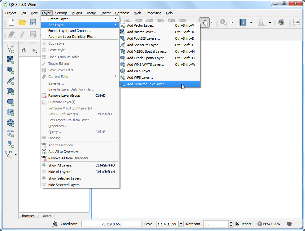
To start, we will import the CSV file into QGIS. (see Mengimpor file Spreadsheet atau CSV. for more details). Click .
Browse to the
2015-08-surrey-street.csvfile on your computer and open it. (Your filename maybe different if you downloaded a fresh copy of the dataset). Select CSV (comma separated values) as the file format. You will see theLongitudeandLatitudecolumns automatically selected as X and Y fields. Make sure you check the Use spatial index option as that will speed up your operations on this layer. Click OK.
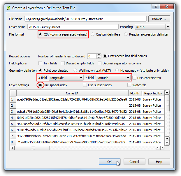
Anda mungkin melihat sejumlah error. Anda dapat tidak menghiraukan hal ini untuk tujuan tutorial ini. Klik Close.
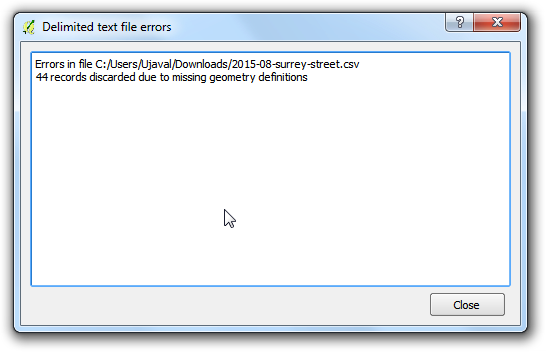
As the data layer is loaded in QGIS, you will see a warning dialog CRS was undefined: defaulting to CRS EPSG:4326 - WGS84. The CSV importer assumes the CRS EPSG:4326 if your coordinates are in Latitude/Longitude. If your X and Y coordinates were in a projected CRS, you will get a dialog prompting you to choose the CRS. As our data is in EPSG:4326, you can ignore the warning.
Catatan
If you need to change the automatically assigned CRS, you can use .
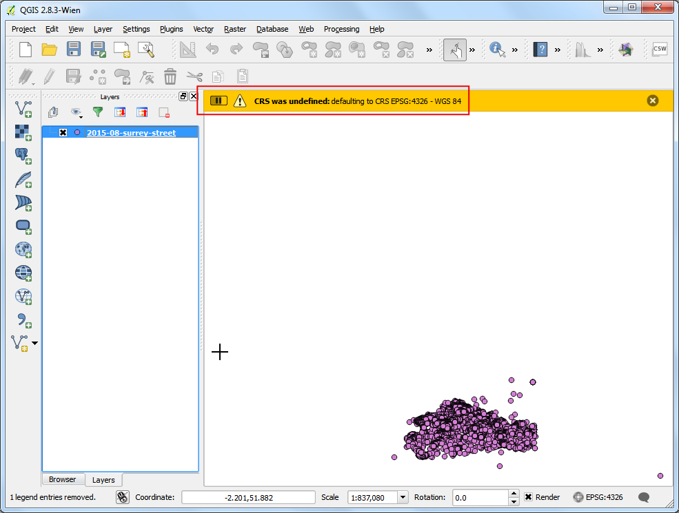
Zoom-in sedikit lebih dekat untuk mendapat visual yang lebih baik pada data. Anda akan melihat bahwa data cukup padat dan sulit untuk tahu di mana konsentrasi tinggi poin-poin tersebut. Ini saatnya heatmap menjadi berguna.
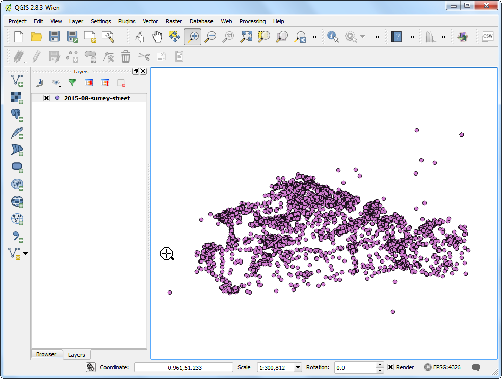
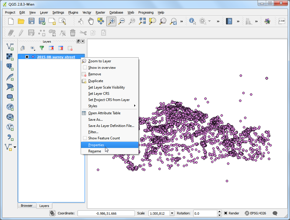
If you need to create a heatmap for purely visual purpose or for printing - QGIS has a built-in symbology renderer called Heatmap. Let's try that first. Right-click on the layer
2015-08-surrey-streetand select Properties.
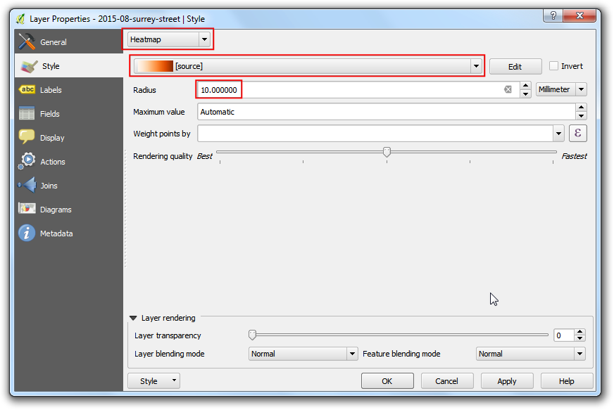
In the Properties dialog, switch to the Style tab. Select Heatmap as the renderer. You have a lot of choice of color-ramps for the heatmap. Choose the
Orangescolor-ramp. Leave the other parameters to default and click OK.
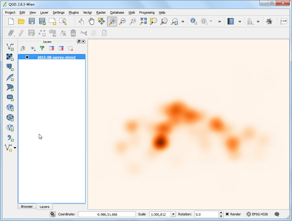
You will see a nice heatmap of your data and pockets of heat where there is a high concentration of crime. There are quite a few options available in the heatmap renderer to create the most appropriate visualization for your dataset. If you just wanted to create a heatmap for print or visual inspection - you are done! But we will explore another more powerful heatmap creation option where you can use the results in your analysis also.
Enable a core plugin named
Heatmap. See Menggunakan Plugins to know how to enable built-in plugins. Once you have enabled the plugin, go to .
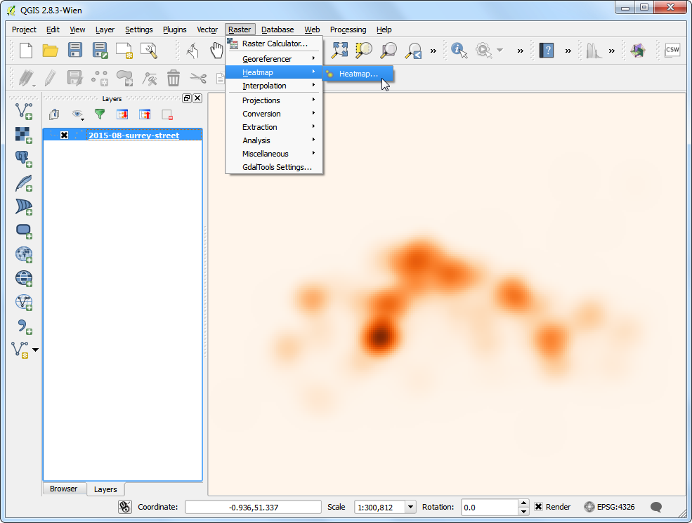
In the Heatmap Plugin dialog, choose
crime_heatmapas the name out the Output raster. Enter 1000 meters as the Radius. Radius is the area around each point that will be used to calculate the i`heat` a pixel received. Check the Advanced so we can specify the output size of our heatmap. Enter2000as Rows value. The Columns value will update automatically. Click OK to start the heatmap creation process.
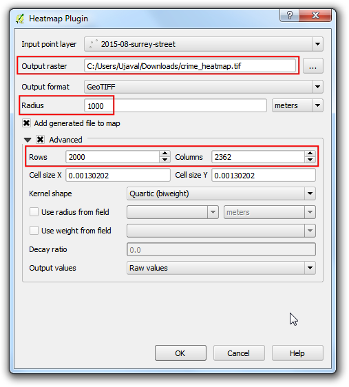
Once the processing is finished, you will see a grayscale layer called
crime_heatmaploaded into the canvas. Uncheck the2015-08-surrey-streetlayer.
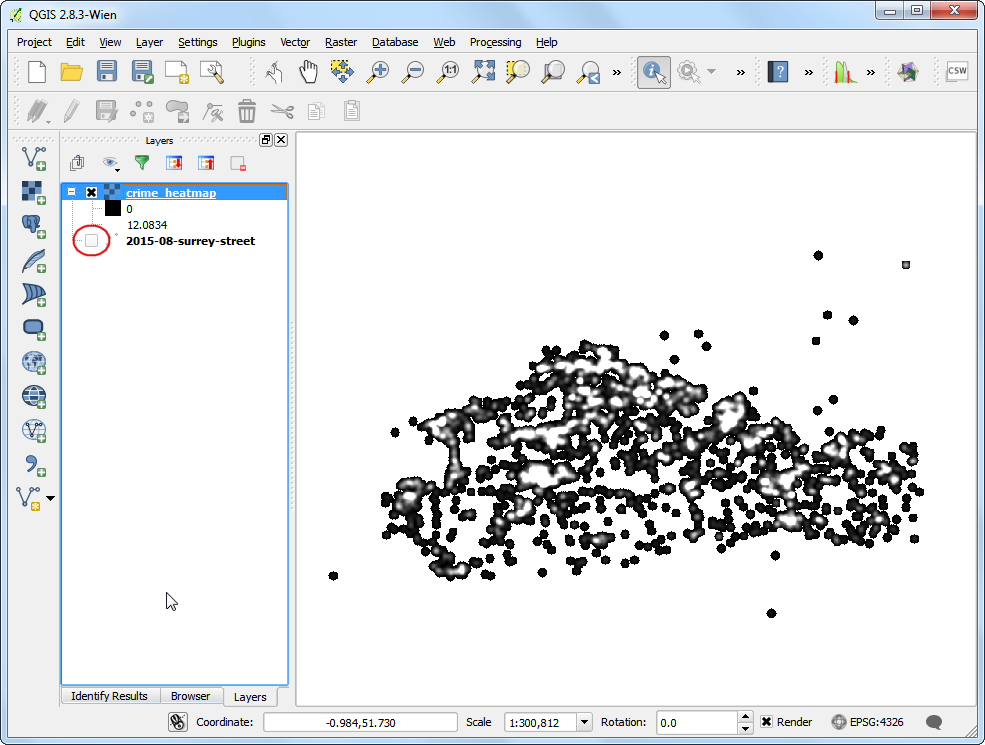
Let's make our heatmap look more like the traditional heatmap similar to the earlier visualization. Right-click on the heatmap layer and click Properties.
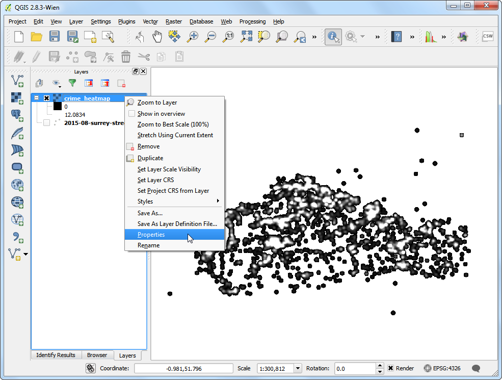
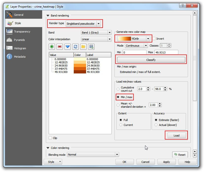
In the Style tab, select Singleband pseudocolor as the Render type. Next, under the section Load min/max values, select the Estimate (faster) as the Accuracy and click Load. This will scan the heatmap and find the minimum and maximum pixel values. These values will be used to generate an appropriate color ramp. In the section Generate new color map, select YlOrRd (Yellow-Orange-Red) as the color ramp, and click Classify. Click OK.
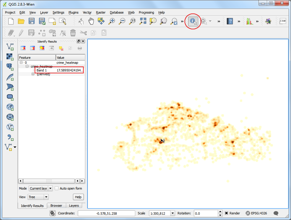
Sekarang anda akan melihatt sebuah heatmap yang lebih menarik . Anda dapat memilih tool xxx dan klik pada pixel manapun pada heatmap. Anda akan melihat nilai pixel pada pop-uo hasil. Nilai pixel ini adalah penghitungan berapa banyak poin dari layer sumber yang masuk pada radius yang sudah ditentukan ( dalam kasus kita - 1000m ) di sekitar pixel.
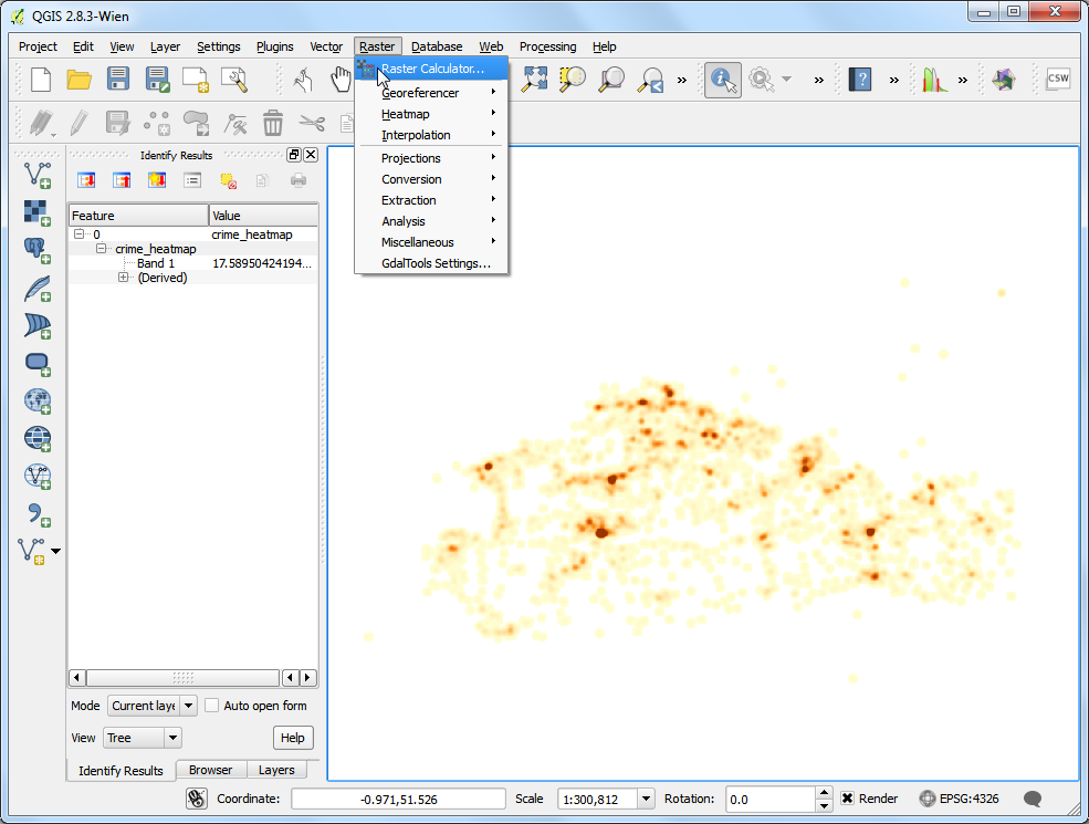
Now you have your heatmap layer that can be saved for future use. Many times, you want to identify the hotspots where there is high-concentration of points. We will now try to identify such hotspots using this heatmap. Go to .
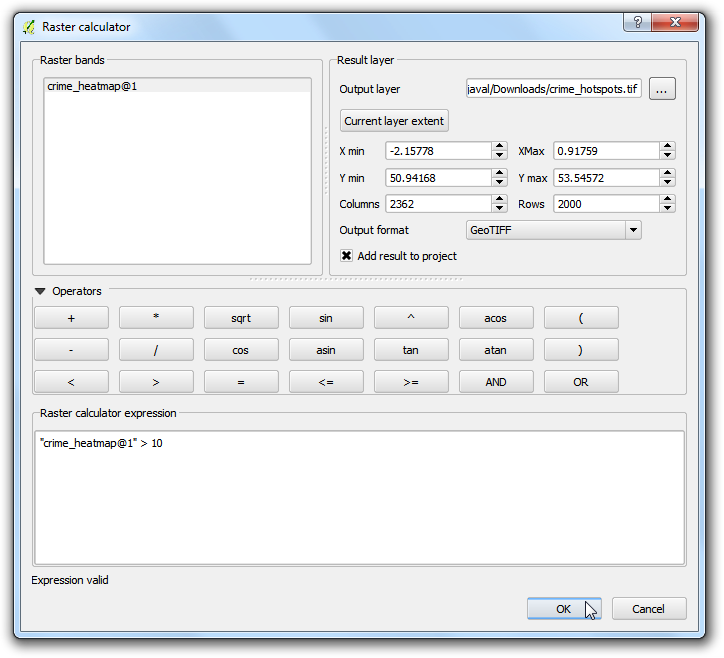
You will have to decide on a threshold value first. All pixel values above that threshold will be considered to be in a cluster. Let's use a value of
10for this data. In Raster calculator dialog, name the output layer ascrime_hotspots_vector. Double-click oncrime_heatmap@1under the Raster bands section and it will be added to the Raster calculator expression textarea. Complete the expression as shown below. Check the box next to Add result to project and OK.
"crime_heatmap@1" > 10
A new layer called
crime_hotspotswill be added to QGIS. This layer has pixels with values of either 0 or 1. All pixels in the input layer where the pixel value was larger than10now have a value of 1 and all remianing pixels are 0. Click on .
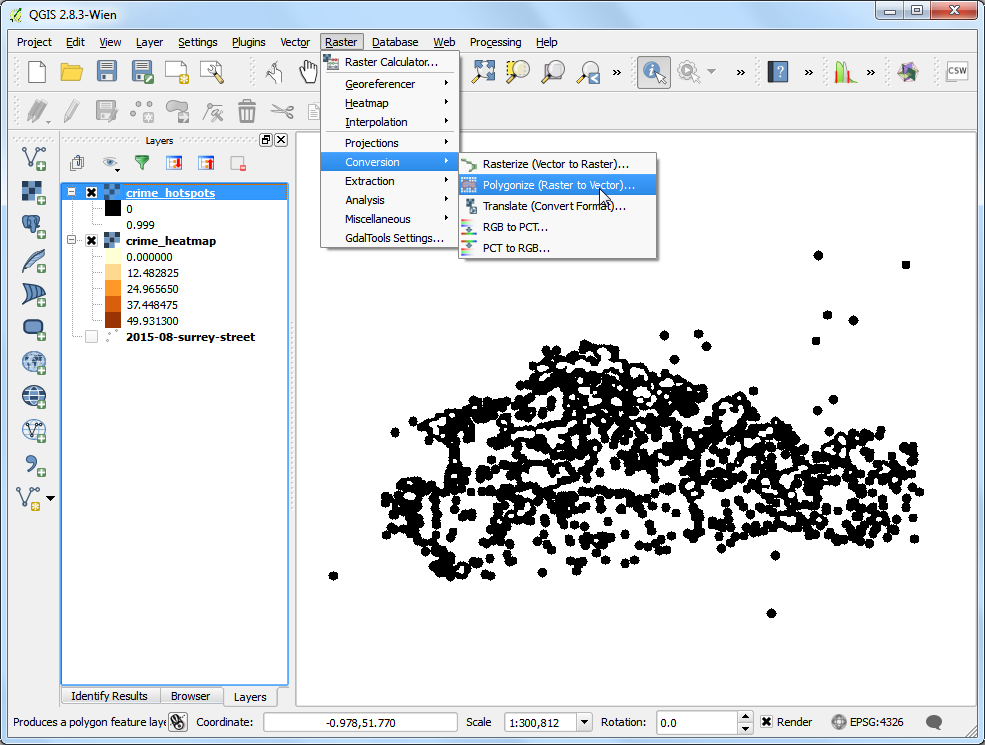
Name the output file as
crime_hotspots_vector. Check the box next to Field name as well as Load into canvas when finished. Click OK.
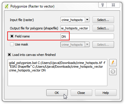
Once the conversion finishes, you will have yet another layer named
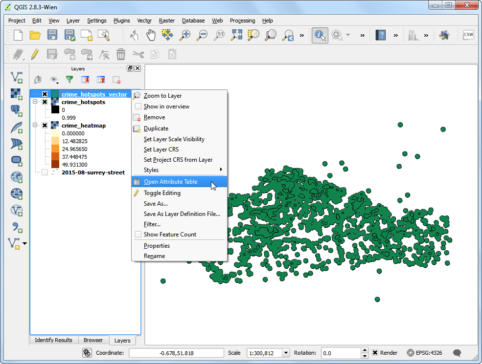
crime_hotspots_vectoradded to QGIS. This is the vector representation of the clusters that were created in the previous step. The layers contain clusters with both 0 and 1 values. Let's filter out the 0 values, so we get the clusters of hotspots. Right-click on the layer and select Open Attribute Table.
Pada Attribute table , klik Select feature using an expression.
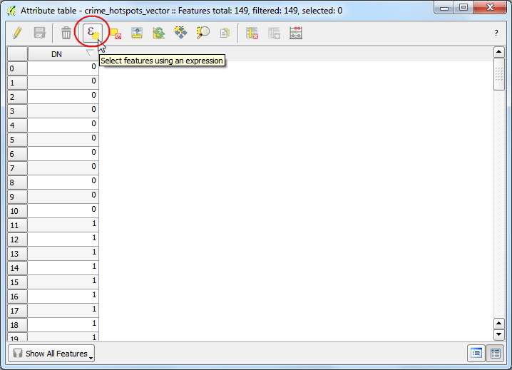
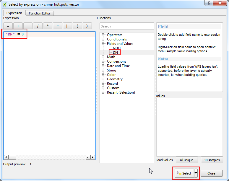
Enter the expression as shown below and click Select. Next, click on Close.
"DN" = 0
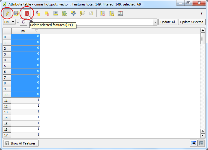
In the main attribute table window, you will see some features highlighted. These are the features that matched our query. Click the Toggle editing mode button in the toolbar and then click the Delete selected features (DEL) button.
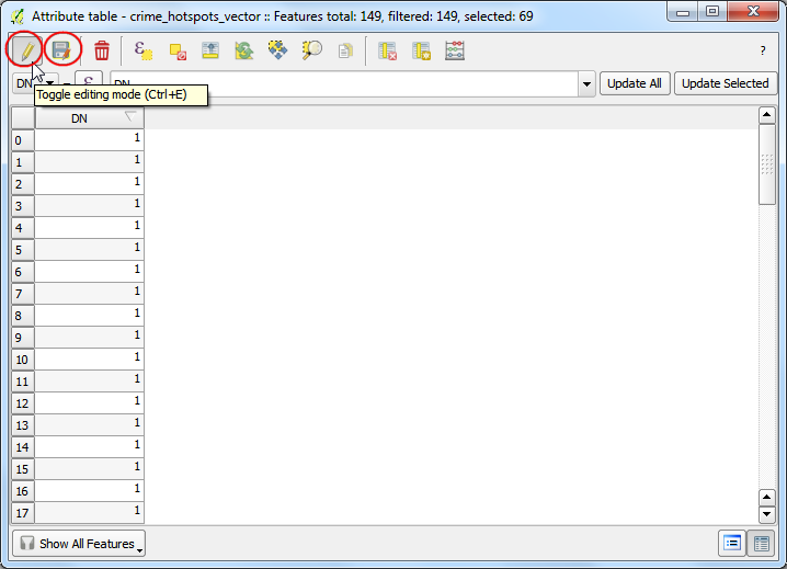
Once the selected features are deleted, click the Save Edits button and then Toggle editing mode again to put the layer in read-only mode. Close the attribute table window.
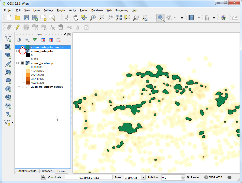
In the main QGIS window, un-check the
crime_hotspotslayer. The final layercrime_hotspots_vectorcontains the cluster extracted from the heatmap. These clusters are the intelligence gathered from the raw data and can provide useful insights as well as serve as an input for further action.
If you want to report any issues with this tutorial, please comment below. (requires GitHub account)