Topological Data Analysis of Genetic Regulatory Circuits
Gary Welz
CopernicusAI / CUNY Graduate Center (PoI)
February 27, 2026
From papers to flowcharts
First attempt at the β-galactosidase flow chart in 1995. This appeared in an article in The X Advisor, an online magazine for Unix developers. The article was entitled “Is the Genome Like a Computer Program?” and contained excerpts from my conversations with biologists on the bionet.genome.chromosome newsgroup. The article was archived at the Wayback Machine (Internet Archive); the newsgroup discussions are archived by Google.
The 1995 chart was created from text alone — the same process LLMs use today. The source was Berg & Singer (1992, pp. 71–73). This shows that diagrams are only as detailed and reliable as their source material; using different sources for the same process can yield different charts.
1995 article (Internet Archive) | Source: Berg, P. & Singer, M. (1992). Dealing With Genes. University Science Books, pp. 71–73.
bionet.genome.chromosome thread: first posting (flowchart with “and”/“or”) · Robbins: “care must be taken in interpreting that flow chart”; “computer-science insights… potentially huge payoffs” · Dellaire: genome structure (not just sequence) encodes how the code is read—context spatial/temporal · Robbins.
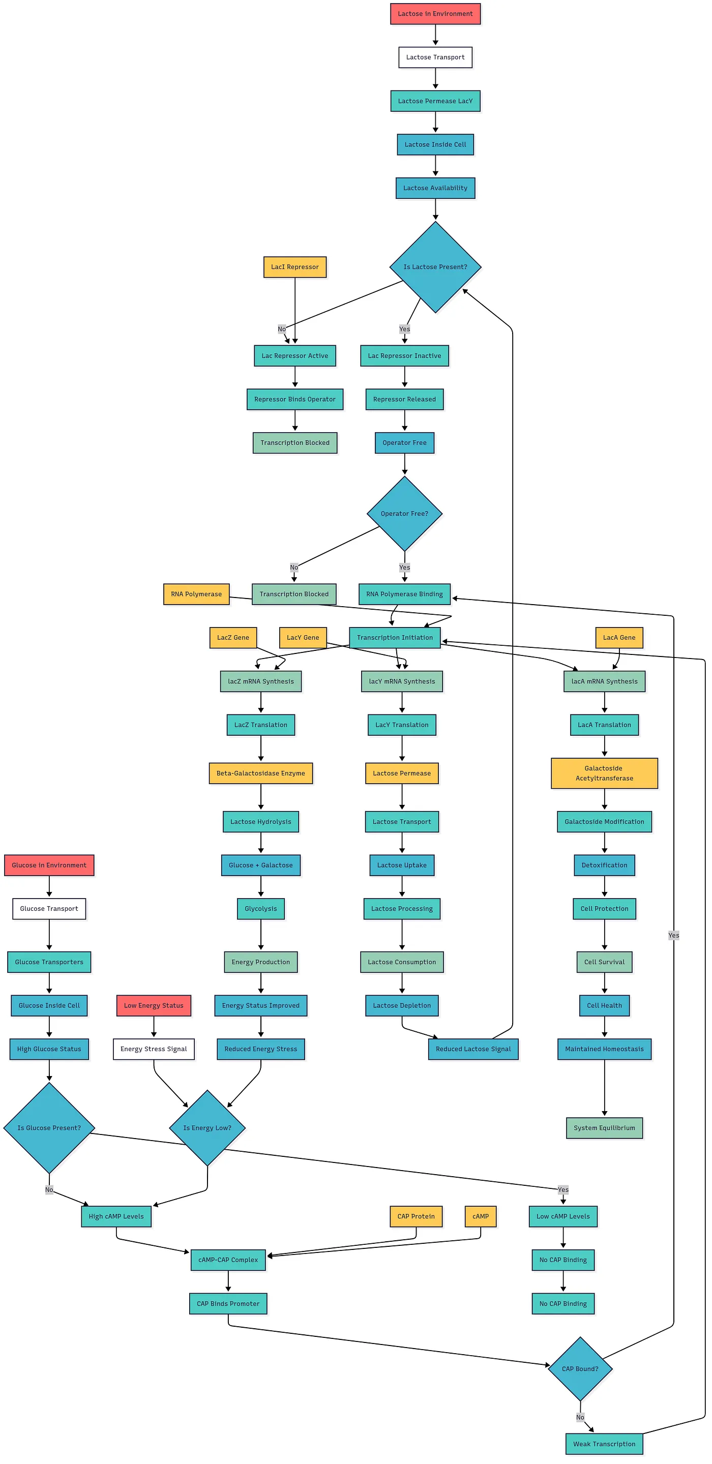
Same chart, 30 years later
This is the same Lac operon / β-galactosidase idea — but generated with LLMs and Mermaid Markdown. The original chart was so time-consuming that the idea sat dormant for decades. Now we can produce any of these flowcharts from a single prompt in seconds.
Traditional TDA starts from numerical data. Here we start from text — paper descriptions — and turn them into visual flowcharts first. That shift is what makes the rest possible.
Traditional TDA: Numerical data → Feature vectors → Topology
This work: Text (papers) → Visual flowcharts → Features → Topology
Key: Mermaid Markdown converts textual process descriptions into structured flowcharts
Flowcharts become visual data; TDA reveals structure
We extract topology from descriptions, not from direct measurements
Novel aspects: Text-to-visual-to-topology pipeline; features include nodes, conditionals (edges), AND/OR gates, and flowchart loops (back-edges); feedback loops = H₁ loops (literal correspondence); LLM-assisted curation at scale. Similar to Politics case study (Carlsson & Vejdemo-Johansson, 2021, pp. 199–201) but with these distinct characteristics.
The Question
We’re asking whether the shape of these circuits — as captured by topology — lines up with what biologists already know: feedback loops, cascades, and regulatory motifs.
Can we detect regulatory structure (feedback, cascades) from circuit topology?
Feedback loops are literally loops — they should appear in H₁
Can text-derived visual data support that?
The GLMP Database
The Genome Logic Modeling Project gives us 108 processes — each one a Mermaid flowchart with nodes, conditionals (edges), and OR/AND logic. We extract five features per process: nodes, conditionals, OR gates, AND gates, and loops (back-edges).
108 genetic regulatory circuits
E. coli (66), S. cerevisiae (38), Bacillus subtilis (4)
Each process: Mermaid flowchart → 5 features (nodes, conditionals, OR, AND, loops)
Each process in GLMP is grounded in literature: the JSON holds PubMed/DOI and the viewer lets anyone suggest improvements. So the flowcharts are citable and correctable.
Each process JSON includes references: PubMed, DOI, sources
Viewer accepts feedback — suggest corrections or improvements
These capture circuit complexity and logic structure
TDA Pipeline
From the feature matrix we build a distance between every pair of processes, then run a Vietoris–Rips filtration and use Ripser to get persistence diagrams. The cocycles tell us which processes sit on which topological loop.
Feature matrix → Euclidean distance
Vietoris-Rips filtration
Ripser (maxdim=2), cocycle extraction
Output: persistence diagrams (H₀, H₁, H₂)
Cocycles tell us which processes form each H₁ loop
What Are We Counting? H₀, H₁, H₂
Before the persistence diagram, a quick intuitive ladder:
H₀ (components): “Are the pieces connected?” — In GLMP, H₀ starts at 108 (one per process) and collapses as the Vietoris–Rips radius grows and processes link up.
H₁ (loops): “Are there feedback loops?” — Closed cycles with no filled-in face. In gene regulation, this is feedback: A→B→C→A with no shortcut. The 33 H₁ features are precisely these unfilled cycles. Biologically richest for GLMP.
H₂ (voids): “Are there enclosed cavities?” — Hollow spheres, interior of a ball. In cancer GRN work (Masoomy et al., 2021), H₂ appeared in healthy cells as redundant, enclosed structures. GLMP yields H₂ = 1 (expected for 108 points in 5D).
Mathematical Note (1): Betti Numbers — History & Geometry
Betti numbers β₀, β₁, β₂ count connected components, loops, and voids. Named for Enrico Betti (1823–1892), formalized by Poincaré (1890s). Geometrically: β₀ = pieces; β₁ = independent loops that don’t bound a filled region; β₂ = enclosed voids. Euler’s formula χ = V − E + F = 2 (planar graphs) — F includes the outer face.
In a planar graph, a face is a region bounded by edges—including the outer, unbounded region. In homology, faces correspond to 2-simplices (filled triangles): three vertices within the distance threshold form a triangle whose interior “fills in” the loop. When a loop is not bounded by any 2-simplex—no triangle fills it in—that loop persists as an H₁ feature. Our 33 H₁ loops are exactly those cycles that fail to be filled; they are the β₁ contribution to χ.
Face = 2-simplex = filled triangle
Loop not bounded by a face → H₁ feature persisting
Persistence Diagram
Here’s the persistence diagram. We get one component per process in H₀, and 33 loops in H₁. The question is whether those H₁ loops line up with known biology — feedback circuits, stress responses, and so on.
H₀: 108 components (one per process)
H₁: 33 loops
H₂: 1 void (expected—few points form persistent 2D cavities)
Key question: Do these loops correspond to biological structure?
What Do the Loops Look Like? (1) PCA + Cocycle Edges
The persistence diagram tells us H₁ has 33 loops, but not where they sit in the data. To make homology visible, we project the 5D feature space to 2D via PCA (principal component analysis—finds directions of maximum variance; preserves distances for visualization), then draw the cocycle edges—the pairs of processes that form each cycle. Each colored loop is one H₁ cycle: red (#1), blue (#2), green (#3), purple (#4), orange (#5). Lac operon, two-component, and SOS are labeled.
Cocycles: which (process A, process B) pairs form each H₁ cycle
Project to 2D via PCA → draw edges between paired processes
The polygons you see are the loops; feedback circuits cluster in them
The Mapper algorithm builds a simplicial complex from the data: cluster nearby processes, then connect clusters that overlap. Each node is a cluster of similar processes (node size = number of processes); edges connect overlapping clusters. Cycles in this graph correspond to topological loops—so the loops in the Mapper graph visualize the H₁ structure in a different way. This complements the persistence diagram and the cocycle-in-PCA view.
The most persistent loop aggregates stress response, protein quality control, and DNA repair: SOS response, quorum sensing, biofilm formation, base excision repair (BER), BAM complex assembly, ribosome assembly, RNA pol recycling, Type III secretion, ubiquitin-proteasome, and unfolded protein response (UPR). E. coli and yeast; shared “stress + quality control + feedback” character.
Common thread: stress, protein quality control, feedback
Cross-organism: E. coli, yeast
Example: SOS Response (Loop #1)
The SOS response is E. coli’s emergency DNA repair system: damage activates RecA, which inactivates LexA repressor, inducing repair genes. Classic feedback — repair turns genes off. SOS sits in the top H₁ loop alongside quorum sensing, biofilm, UPR, and protein quality control — processes that share stress-response and feedback structure.
Six processes: antibiotic efflux pumps, arginine biosynthesis, osmotic stress response, tryptophan biosynthesis, peroxisome biogenesis, vacuolar protein sorting. Metabolic regulation and organelle biogenesis — E. coli and yeast. Topology groups by circuit structure: feedback in biosynthesis and stress-induced transport.
Five processes: ara operon, maltose regulon, Pho regulon, nitrogen catabolite repression (NCR/TORC1), competence development. Nutrient and developmental regulation — ara and Pho are classic feedback circuits; topology groups by nutrient-sensing regulatory logic. Cross-organism: E. coli, yeast, Bacillus.
AraC acts as repressor or activator depending on arabinose; DNA looping and CRP–cAMP integration. Ara sits in Loop #5 with Pho regulon, maltose regulon, nitrogen catabolite repression, and competence — all nutrient-sensing or developmental decisions with shared regulatory logic.
With the new loop-based feature set, known feedback circuits cluster in coherent loops: SOS, quorum sensing, biofilm in Loop #1 (stress + feedback); ara and Pho in Loop #5 (nutrient-sensing feedback); trp biosynthesis in Loops #2 and #4. Topology recovers regulatory structure — stress, protein quality, nutrient regulation — from structural features alone.
SOS, quorum sensing, biofilm → Loop #1
Ara operon, Pho regulon → Loop #5
Trp biosynthesis → Loops #2, #4
Interpretation: topology captures stress, nutrient-sensing, and feedback architecture
Organism Patterns
All top five loops mix organisms. Loop #1: E. coli and yeast. Loops #2, #3: E. coli and yeast. Loop #4 and #5: E. coli, yeast, and Bacillus. Topology groups by circuit structure, not by species — regulatory logic transcends organism boundaries.
Loop #1, #2, #3: E. coli + yeast
Loop #4, #5: E. coli + yeast + Bacillus
Regulatory logic is shared across organisms
Why These Features Work
Using loop (back-edge) features instead of NOT gates yields richer persistence values and clearer biological groupings. The coherence check asks whether topology recovers known biology — not the reverse.
Known feedback circuits cluster coherently: stress in Loop #1, nutrient-sensing in Loop #5, metabolic feedback in Loops #2 and #4.
Conclusion: loop-based features capture coarse regulatory topology. The new feature set is a distinct experiment; results are richer and more interpretable.
Limitations and Caveats
Sample size: 108 processes — enough to reveal structure, but scaling to 200–500+ is a priority.
Feature sensitivity: Five features: nodes, conditionals (edges), OR gates, AND gates, loops. Ablation shows node_count is most load-bearing; coherence is distributed across features, not a single-feature artifact.
Graph-theoretic enrichment: cycle rank, longest path length, AND/OR gate ratios — planned for next pipeline iteration.
LLM-generated flowcharts require expert fact-checking; the GLMP viewer feedback mechanism is one avenue for community validation.
Open question: Does topology predict regulatory function, or correlate with known biology? The coherence check supports the latter; prediction requires prospective validation.
Next Steps
We’re moving toward Mapper, ablation and null-model validation, and richer features. A longer-term goal is to use flowcharts and TDA as a kind of Rosetta Stone: linking topological structure to the genetic “machine code” on the chromosome — the sequence motifs that implement AND/OR connectives.
Rosetta Stone goal: Topology → shared regulatory sequence motifs (binding-site logic for AND/OR) — falsifiable if circuits in the same H₁ loop share enriched motifs
Mapper: circuit classes as nodes
Feature ablation study: rerun TDA dropping one feature at a time to test H₁ loop stability
Null model permutation test (n=1,000): p = 0.022 — significant at p < 0.05
Graph-theoretic features: cycle rank, longest path, gate ratios — planned for next pipeline iteration
Persistent cohomology: circular coordinates for feedback depth
Scaling: 200–500+ genetic circuits
Biologist validation of flowcharts; CUNY TDA seminar group
Open source: github.com/garywelz/glmp/tree/main/tda-analysis
References
Carlsson, G. & Vejdemo-Johansson, M. (2021). Topological Data Analysis with Applications. Cambridge University Press.
Bauer, U. (2021). Ripser: efficient computation of Vietoris–Rips persistence barcodes. J. Appl. Comput. Topol. 5, 391–423.
Berg, P. & Singer, M. (1992). Dealing With Genes. University Science Books.
Masoomy, H., et al. (2021). Topological analysis of interaction patterns in cancer-specific gene regulatory network. Sci. Rep. 11, 16414.
Rivera-Cancel, G., et al. (2014). Full-length structure of a monomeric histidine kinase reveals basis for sensory regulation. PNAS 111(50), 17839–17844.
Swingle, D., et al. (2025). Variations in kinase and effector signaling logic in a bacterial two component signaling network. J. Biol. Chem. 301, 108534.
Tralie, C., Saul, N., & Bar-On, R. (2018). Ripser.py: A lean persistent homology library for Python. J. Open Source Softw. 3(29), 925.
Welz, G. (1995). Is the genome like a computer program? The X Advisor (July 1995). Internet Archive.
Acknowledgments and Questions
Jordan Matuszewski; CUNY Graduate Center TDA seminar group
Kevin Gardner and colleagues (ASRC, CCNY) — two-component signaling and kinase/effector logic