Marine Finfish Aquacultural Production

Summary

Supporting the production of aquacultured fish and shellfish is an important service provided by coastal and marine environments. Because salmon is one of the two most important finfish in aquaculture worldwide, the current version of the InVEST aquaculture model analyzes the volume and economic value of Atlantic salmon (Salmo salar) grown in netpen aquaculture facilities based on farming practices, water temperature, and economic factors. Inputs for the present model include farm location, management practices at the facilities, water temperature, economic data for valuation, and the time period over which results are of interest. This model is best used to evaluate how human activities (e.g., the addition or removal of farms or changes in harvest management practices) and climate change (e.g., change in sea surface temperature) may affect the production and economic value of aquacultured Atlantic salmon. Limitations of the model include assumptions that harvest practices, prices, and costs of production of aquacultured fish are constant for the selected time period. Additionally, risk of disease outbreaks and variability between individual salmon within a farm are not included in the model.

Introduction

Human demand for protein from the ocean has rapidly increased and is projected to continue to do so in coming decades (Delgado et al. 2003, Halwart et al. 2007, Soto et al. 2008). In recent years, the scales, previously tilted towards provisioning of protein from capture fisheries, have shifted toward aquaculture (Griffin et al., 2015). In particular, finfish aquaculture, primarily for Atlantic salmon, has intensified in coastal areas over the past two decades (FAO 2004, Goldburg and Naylor 2004, Naylor and Burke 2005). In 2002, farmed salmon production, over 90% of which was for Atlantic salmon, was 68% higher than the volume of wild capture (FAO 2004). Atlantic salmon farming, conducted in floating netpens in low energy, nearshore areas, is a well-established, consolidated industry that operates in the temperate waters of Norway, Chile, the United Kingdom and Canada.

Commercial operations for Atlantic salmon use the marine environment to produce a valuable commodity, which generates revenue and is a source of employment. Yet salmon farming is controversial due to potentially adverse impacts to marine ecosystems and, thereby, people who derive their livelihoods from those ecosystems (e.g., commercial fishermen, tourism operators). Concerns about the effects of Atlantic salmon aquaculture on the marine ecosystem involve debate about the impacts of emission of dissolved and solid wastes to water quality and living habitats, degradation of water quality due to use of antibiotics, mixing and competition of escaped farmed salmon with endemic species (e.g., Pacific salmon), increased risk of parasitism and disease, and depletion of forage fish resources harvested from other ecosystems for use as Atlantic salmon feed.

Regulations for the Atlantic salmon aquaculture industry vary regionally, from the most stringent requirements for locating and operating facilities in Norwegian waters, to fewer constraints for farms in Chilean waters. For all operations, there are regulatory limits on where and how aquaculture can be conducted and requirements for monitoring and regulating the amount of waste generated at different facilities, and in some cases, mitigation requirements.

Weighing the economic benefits of Atlantic salmon aquaculture against the environmental costs involves quantifying both. The InVEST model presented here does the former by quantifying the volume and economic value of the commodity.

The Model

The model is designed to address how the production and economic value of farmed Atlantic salmon at individual aquaculture facilities and across a user-defined study area change depending on farm operations and changes in water temperature. Temporal shifts in price, costs or harvest management practices are not dynamically modeled, but can be represented by running the model sequentially, where each run uses different information on prices, costs and farm operations. The risk of disease outbreaks and variability between individual salmon within a farm are not included in the model. The model will yield the most accurate outputs when parameterized with site-specific temperature and farm operations data. If site-specific data are unavailable, the provided ranges of default values can be used to yield first approximations of results (see Data Needs section).

The model is run simultaneously for all Atlantic salmon farms identified by the user. Each farm can have a user-defined set of operations and management practices. The volume of fish produced on a farm depends on water temperature (which affects growth), the number of fish on the farm, the target harvest weight range, and the mortality rate. Fish growth is modeled on a daily time-step until the fish reach the target harvest weight range, after which they are harvested. After a user-defined fallowing period, the farm is restocked and this initiates the next production cycle. Production cycles continue for each farm until the end of the time period of interest (e.g., 2 years, 10 years). Outputs include the harvested weight of fish and net revenue per cycle for each individual farm. In addition, the model yields a map of the total harvested weight, total net revenue, and net present value over the time period of interest.

How it Works

The model runs on a vector GIS dataset that maps individual aquaculture facilities for Atlantic salmon that are actively farmed over a user-defined time period. The map can be based on current farming (the “status quo” or “baseline” scenario), or on scenarios of projected expansion or contraction of the industry or on projected changes in water temperature.

In each farm we model the production of fish in three steps. (1) We model the growth of individual fish to harvest weight. (2) We calculate the total weight of fish produced in each farm as the number of fish remaining at harvest, multiplied by their harvested weight, less the weight removed during processing (gutting, etc.) and the weight of fish lost to natural mortality. (3) Lastly, all the fish in a farm are harvested at the same time, and the farm is restocked after a user-defined fallowing period. Valuation of processed harvest is an optional fourth step in the model.

Growth of the Individual Fish to Harvest Weight

Atlantic salmon weight (kg) is modeled from size at outplanting to target harvest weight. Weight is a function of growth rate and temperature (Stigebrandt 1999). Outplanting occurs when Atlantic salmon have been reared beyond their freshwater life stages. The model runs on a daily time step. Fine resolution temporal data are more appropriate for the seasonal evaluation of environmental impacts (e.g., seasonal eutrophication).

Weight \(W_t\) at time \(t\) (day), in year \(y\), and on farm \(f\) is modeled as:

(1)\[W_{t,y,f} = { ({\alpha W_{t-1,y,f}^\beta \cdot e^{T_{t-1,f} \tau}}) + W_{t-1,y,f} }\]

where \(\alpha\) (g^1-bday^-1) and \(\beta\) (non-dimensional) are growth parameters, \(T_{t,f}\) is daily water temperature (C) at farm \(f\), and \(\tau\) (C^-1) represents the change in biochemical rates in fishes with an increase in water temperature. The value for Atlantic salmon (0.08) indicates a doubling in growth with an 8-9 C increase in temperature. Daily water temperatures can be interpolated from monthly or seasonal temperatures. The growing cycle for each farm begins on the user-defined date of outplanting (\(t=0\)). The outplanting date is used to index where in the temperature time series to begin. The initial weight of the outplanted fish for each farm is user-defined. An individual Atlantic salmon grows until it reaches its target harvest weight range, which is defined by the user as a target harvest weight.

Total Weight of Fish Produced per Farm

To calculate the total weight of fish produced for each farm, we assume that all fish on a farm are homogenous and ignore variability in individual fish growth. This assumption, though of course incorrect, is not likely to affect the results significantly because 1) netpens are stocked so as to avoid effects of density dependence and 2) aquaculturists outplant fish of the same weight to netpens for ease of feeding and processing. We also assume that when fish reach a certain size, all fish on the farm are harvested. In practice, farms consist of several individual netpens, which may or may not be harvested simultaneously. If a user has information about how outplanting dates and harvest practices vary between netpens on a farm, the user can define each netpen as an individual “farm.”

The total weight of processed fish \(TPW\) on farm \(f\) in harvest cycle \(c\):

(2)\[TPW_{f,c} = { W_{t_h,h,f} \cdot d \cdot n_f e^{-M \cdot (t_h - t_0)} }\]

where \(W_{t_h,h,f}\) is the weight at date of harvest \(t_h,y\) on farm \(f\) from Equation (1), \(d\) is the processing scalar which is the fraction of the fish in the farm that remains after processing (e.g., weight of headed/gutted or filleted fish relative to harvest weight), \(n_f\) is the user-defined number of fish on farm \(f\), and \(e^{-M \cdot (t_h - t_o)}\) is the daily natural mortality rate \(M\) experienced on the farm from the date of outplanting (\(t_0\)) to date of harvest (\(t_h\)).

Restocking

The previous 2 steps describe how fish growth is mdoeled for one production cycle. However, the user may want to evaluate production of fish over a series of production cycles. The primary decision to be made when modeling multiple harvest cycles is if (and if so, how long) a farm will be left to lie fallow after harvest and before the next production cycle begins (initiated by outplanting).

If used, fallowing periods are considered hard constraints in the model such that a farm cannot be restocked with fish until it has lain fallow for the user-defined number of days. This is because fallowing periods are often used to meet regulatory requirements, which can be tied to permitting, and thus provide incentive for compliance. Once fish are harvested from a farm and after the user-defined fallowing period, new fish are outplanted to the farm. The model estimates the harvested weight of Atlantic salmon for each farm in each production cycle. The total harvested weight for each farm over the time span of the entire model run is the sum of the harvested weights for each production cycle.

Valuation of Processed Fish (Optional)

The aquaculture model also estimates the value of that harvest for each farm in terms of net revenue and net present value (NPV) of the harvest in each cycle. The net revenue is the harvest weight for each cycle multiplied by market price, where costs are accounted for as a fraction of the market price for the processed fish. Fixed and variable costs, including costs of freshwater rearing, feed, and processing will be more explicitly accounted for in the next iteration of this model. The NPV of the processed fish on a farm in a given cycle is the discounted net revenue such that:

(3)\[NPV_{f,c} = { TPW_{f,c} {[{p (1-C)]} \cdot {1\over {{(1+r)}^t}}} }\]

where \(TPW_{f,c}\) is the total weight of processed fish on farm \(f\) in harvest cycle \(c,p\) is the market price per unit weight of processed fish, \(C\) is the fraction of \(p\) that is attributable to costs, \(r\) 1 is the daily market discount rate, and \(t\) is the number of days since the beginning of the model run.

Note

The beginning of the model run is the initial outplanting date for the very first farm (of all the farms in the study area) to receive fish. Thus, the net revenue for each farm in each harvest cycle is discounted by the number of days since the very first farm was initially stocked. The total NPV for each farm over the duration of the model run is the discounted net revenue from each harvest cycle summed over all harvest cycles \(c\).

The discount rate reflects society’s preference for immediate benefits over future benefits (e.g., would you rather receive $10 today or $10 five years from now?). The default annual discount rate is 7% per year, which is one of the rates recommended by the U.S. government for evaluation of environmental projects (the other is 3%). However, this rate can be set to reflect local conditions or can be set to 0%.

Uncertainty Analysis (Optional)

Optionally, if the fish growth parameters are not known with certainty, the model can perform uncertainty analysis. This uncertainty analysis is done via a Monte Carlo simulation. In this simulation, the growth parameters (\(\alpha\) and \(b\)) are repeatedly sampled from a given normal distribution, and the model is run for each random sampling.

The results for each run of the simulation (harvested weight, net present value, and number of completed cycles per farm) are collected and then analyzed. Uncertainty results are output in two ways: first, the model outputs numerical results, displaying the mean and the standard deviation for all results across all runs. Second, the model creates histograms to help visualize the relative probability of different outcomes. (After version 3.8.0, histograms are no longer generated by the model due to instability in the plotting library.)

Limitations and Simplifications

Limitations of the model include assumptions that harvest practices, prices, and costs of production of aquacultured fish are constant over the selected time period. Additionally, risk of disease outbreaks and variability between individual salmon within a farm are not included in the model.

The current model operates at a daily time step (requiring daily temperature data).

Uncertainty in input data is currently supported only for fish growth parameters. There is currently no support for uncertainty in input data such as water temperature.

Growth is assumed to be exponential up to the point of harvesting. Survival and growth do not depend on density. The assumption is that aquaculturists are optimizing the stocking density such that there is not excess mortality due to over-crowding.

Data Needs

Data Sources

Here we outline the specific data and inputs used by the model and identify potential data sources and default values. Four data layers are required, and one is optional (but required for valuation).

1. Workspace Location (required). Users are required to specify a workspace folder path. It is recommended that the user create a new folder for each run of the model. For example, by creating a folder called “runBC” within the “Aquaculture” folder, the model will create “intermediate” and “output” folders within this “runBC” workspace. The “intermediate” folder will compartmentalize data from intermediate processes. The model’s final outputs will be stored in the “output” folder.:

   Name: Path to a workspace folder.  Avoid spaces.
   Sample path: \InVEST\Aquaculture\runBC
   

2. Finfish Farm Location (required). A GIS polygon or point dataset, with a latitude and longitude value and a numerical identifier for each farm.:

   Names: File can be named anything, but no spaces in the name
   File type: polygon shapefile or .gdb
   Rows: each row is a specific netpen or entire aquaculture farm
   Columns: columns contain attributes about each netpen (area, location, etc.).
   Sample data set: \InVEST\Aquaculture\Input\Finfish_Netpens.shp
   

Note

The user must ensure that one field contains unique integers. This field name (i.e. “FarmID” in the sample data) must be chosen by the user for input #3 as the “farm identifier name”.

Note

The model checks to ensure that the finfish farm location shapefile is projected in meters. If it is not, the user must re-project it before running the model.

3. Farm Identifier Name (required). The name of a column heading used to identify each farm and link the spatial information from the GIS features (input #2) to subsequent table input data (farm operation and daily water temperature at farm tables, inputs # 6-7). Additionally, the numbers underneath this farm identifier name must be unique integers for all the inputs (#2, 6, & 7).:

   Names: A string of text identifying a column in the Finfish Farm Location shapefile's attribute table
   File type: Drop-down option
   Sample: FarmID
   

4. Fish growth parameters (required, defaults provided). Default a (0.038 g/day), b (0.6667 dimensionless units), and \(\tau\) (0.08 C^-1) are included for Atlantic salmon, but can be adjusted by the user as needed. If the user chooses to adjust these parameters, we recommend using them in the simple growth model (Equation (1)) to determine if the time taken for a fish to reach a target harvest weight typical for the region of interest is accurate.:

   Names: A numeric text string (floating point number)
   File type: text string (direct input to the ArcGIS interface)
   Sample (default): 0.038 for a / 0.6667 for b
   

5. Uncertainty analysis data (optional). These parameters are required only if uncertainty analysis is desired. Users must provide three numbers directly through the tool interface.:

• Standard deviation for fish growth parameter a. This represents uncertainty in the estimate for the value of a.

• Standard deviation for fish growth parameter b. This represents uncertainty in the estimate for the value of b.

• Number of Monte Carlo simulation runs. This controls the number of times that the parameters are sampled and the model is run, as part of a Monte Carlo simulation. A larger number will increase the reliability of results, but will also increase the running time of the model. Monte Carlo simulations typically involve about 1000 runs.

6. Daily Water Temperature at Farm Table (required). Users must provide a time series of daily water temperature (C) for each farm in data input #1. When daily temperatures are not available, users can interpolate seasonal or monthly temperatures to a daily resolution. Water temperatures collected at existing aquaculture facilities are preferable, but if unavailable, users can consult online sources such as NOAA’s 4 km AVHRR Pathfinder Data and Canada’s Department of Fisheries and Oceans Oceanographic Database. The most appropriate temperatures to use are those from the upper portion of the water column, which are the temperatures experienced by the fish in the netpens.:

   Table Names: File can be named anything, but no spaces in the name
   File type: *.xls or .xlsx (if user has MS Office 2007 or newer)
   Rows: There are 365 rows (rows 6-370), each corresponding to a day of the year.
   Columns: The first two columns contain the number for that year (1-365) and day-month.
   Sample: \InVEST\Aquaculture\Input\Temp_Daily.xls\WCVI$
   

Note

For clarification on rows, please refer to the sample temperature dataset in the InVEST package (Temp_Daily.xls).

Note

Column “C” and then all others to its right contain daily temperature data for a specific farm, where the numbers found in row 5 must correspond to the numbers underneath the farm identifier name found in input #2’s attribute table.

7. Farm Operations Table (required). A table of general and farm-specific operations parameters. Please refer to the sample data table for reference to ensure correct incorporation of data in the model. If you would like to use your own dataset, you can modify values for farm operations (applied to all farms) and/or add new farms (beginning with row 32). However, do not modify the location of cells in this template. If for example, you choose to run the model for three farms only, they should be listed in rows 10, 11 and 12 (farms 1, 2, and 3, respectively). Several default values that are applicable to Atlantic salmon farming in British Columbia are also included in the sample data table. The majority of these values can be found by talking to aquaculturists in the study area or through regional industry reports from major aquaculture companies (e.g. Panfish, Fjord Seafood, Cermaq, Marine Harvest, Mainstream Canada, and Grieg).

   The General Operation Parameters of the input table includes the following inputs that apply to all farms: + Fraction of the fish weight (in the farm) remaining after processing (e.g., weight of headed/gutted fish relative to harvest weight) + Natural mortality rate on the farm (daily) + Duration of simulation (in years)

   The Farm-Specific Operation Parameters of the input table includes the following inputs:

   • Rows: Each row in this table (table begins at row #10) contains the input data for a specific farm.

   • Columns: Each column contains values and should be named as follows:

     • Farm #: a series of consecutive integers (beginning with “1” in row 10) that identifies each farm and must correspond to the unique integers underneath the farm identifier name found in input #2’s attribute table.

     • Weight of fish at start (kg): this is the weight of fish when they are outplanted, which occurs when Atlantic salmon have been reared beyond their freshwater life stages.

     • Target weight of fish at harvest (kg)

     • Number of fish in farm (absolute)

     • Start day for growing (Julian day of the year): this is the date of the initial outplanting at the start of the model run. Outplanting date will differ in subsequent cycles depending on lengths of growth and fallowing periods.

     • Length of fallowing period (number of days): if there is no fallowing period, set the values in this column to “0”.

Table Names: File can be named anything, but no spaces in the name
File type: *.xls or .xlsx (if user has MS Office 2007 or newer)
Sample: \InVEST\Aquaculture\Input\Farm_Operations.xls\WCVI$

8. Run Valuation? (optional). By checking this box, users request valuation analysis.

9. Valuation parameters (required for valuation, defaults provided).:

   Names: A numeric text string (positive integer or floating point number)
   File type:  text string (direct input to the ArcGIS interface)
   Sample (default):
     a. Market price per kilogram of processed fish.
        Default value is 2.25 $/kilogram
        (Urner-Berry monthly fresh sheet reports on price of farmed Atlantic salmon)
     b. Fraction of market price that accounts for costs rather than profit.
        Default value is 0.3 (30%).
     c. Daily market discount rate.
        We use a 7% annual discount rate, adjusted to a daily rate of 0.000192 for 0.0192% (7%/365 days).
   

Note

If you change the market price per kilogram, you should also change the fraction of market price that accounts for costs to reflect costs in your particular system.

Running the Model

The model is available as a standalone application accessible from the Windows start menu. For Windows 7 or earlier, this can be found under All Programs -> InVEST |version| -> Finfish Aquaculture. Windows 8 users can find the application by pressing the windows start key and typing “finfish” to refine the list of applications. The standalone can also be found directly in the InVEST install directory under the subdirectory invest-3_x86/invest_pollination.exe.

Viewing Output from the Model

Upon successful completion of the model, a file explorer window will open to the output workspace specified in the model run. This directory contains an output folder holding files generated by this model. Those files can be viewed in any GIS tool such as ArcGIS, or QGIS. These files are described below in Section Interpreting Results.

Interpreting Results

Model Outputs

The following is a short description of each of the outputs from the Aquaculture tool. Each of these output files is automatically saved in the “Output” folder that is saved within the user-specified workspace directory:

Final results are found in the output folder of the workspace for this model. The model produces two main output files:

• Output\Finfish_Harvest.shp: Feature class (copy of input 2) containing three additional fields (columns) of attribute data.

  • Tot_Cycles – The number of harvest cycles each farm completed over the course of the simulation (duration in years)

  • Hrvwght_kg – Total processed weight (in kg, Eqn. 2,) for each farm summed over the time period modeled

  • NPV_USD_1k – The discounted net revenue from each harvest cycle summed over all harvest cycles (in thousands of $). This value will be a “0” if you did not run the valuation analysis.

• Output\HarvestResults_[date and time].html: An HTML document containing tables that summarize the inputs and outputs of the model.

  • Farm Operations – a summary of the user-provided input data including: Farm ID Number, Weight of fish at start, Weight of fish at harvest, Number of fish in farm, start day for growing and Length of fallowing period

  • Farm Harvesting – a summary table of each harvest cycle for each farm including: Farm ID Number, Cycle Number, Days Since Outplanting Date, Harvested Weight, Net Revenue, Net Present Value, Outplant Day, Year

  • Farm Result Totals – a summary table of model outputs for each farm including: Farm ID Number, Net Present Value, Number of completed harvest cycles, Total volume harvested

  • Uncertainty Analysis Results – this section will be included only if uncertainty analysis was performed. It includes two parts:

    • Numerical Results – a table summarizing mean and standard deviation for model outputs such as harvested weight, net present value, and number of completed harvest cycles.

    • Histograms – After version 3.8.0, histograms are no longer generated by the model due to instability in the plotting library.

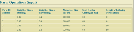
Figure 1: First few rows of a sample Farm Operations table in HTML output

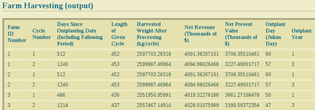
Figure 2: First few rows of a sample Farm Harvesting table in HTML output

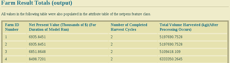
Figure 3: First few rows of a sample Farm Result Totals table in HTML output

Parameter Log

• Each time the model is run a text file will appear in the workspace folder. The file will list the parameter values for that run and be named according to the date and time.

References

Delgado, C., N. Wada, M. Rosegrant, S. Meijer, and M. Ahmed. 2003. Outlook for Fish to 2020: Meeting Global Demand. Washington, DC: Int. Food Policy Res. Inst.

FAO. 2004. Fishstat Plus. Universal software for fishery statistical series. Capture production 1950 - 2004. FAO Fish. Aqua. Dept., Fish. Inf., Data, Stat. Dep.

Goldburg R., and R. Naylor. 2004. Future seascapes, fishing, and fish farming. Front. Ecol. 3:21–28.

Griffin, R., Buck, B., and Krause, G. 2015. Private incentives for the emergence of co-production of offshore wind energy and mussel aquaculture. Aquaculture, 346, 80-89.

Halwart, M., D. Soto, and J.R. Arthur, J.R. (eds.) 2007. Cage aquaculture – Regional reviews and global overview. FAO Fisheries Technical Paper. No. 498. Rome, FAO. 241 pp.

Naylor, R., and M. Burke. 2005. Aquaculture and Ocean Resources: Raising Tigers of the Sea. Ann. Rev. Envtl. Res. 30:185-218.

Soto, D., J. Aguilar-Manjarrez, and N. Hishamunda (eds). 2008. Building an ecosystem approach to aquaculture. FAO/Universitat de les Illes Balears Expert Workshop. 7–11 May 2007, Palma de Mallorca, Spain. FAO Fisheries and Aquaculture Proceedings. No. 14. Rome, FAO. 221p.

Stigebrandt, A., 1999. Turnover of energy and matter by fish—a general model with application to salmon. Fisken and Havet No. 5, Institute of Marine Research, Norway. 26 pp.

Footnotes

1

The daily discount rate is computed as the annual discount rate divided by 365. For an annual discount rate of 7%, the daily discount rate is 0.00019178.