{
"cells": [
{
"cell_type": "markdown",
"metadata": {
"id": "9teObmxrP0FE"
},
"source": [
"##### Copyright 2021 The TensorFlow Authors."
]
},
{
"cell_type": "code",
"execution_count": null,
"metadata": {
"cellView": "form",
"id": "mz8tfSwOP4fW"
},
"outputs": [],
"source": [
"#@title Licensed under the Apache License, Version 2.0 (the \"License\");\n",
"# you may not use this file except in compliance with the License.\n",
"# You may obtain a copy of the License at\n",
"#\n",
"# https://www.apache.org/licenses/LICENSE-2.0\n",
"#\n",
"# Unless required by applicable law or agreed to in writing, software\n",
"# distributed under the License is distributed on an \"AS IS\" BASIS,\n",
"# WITHOUT WARRANTIES OR CONDITIONS OF ANY KIND, either express or implied.\n",
"# See the License for the specific language governing permissions and\n",
"# limitations under the License."
]
},
{
"cell_type": "markdown",
"metadata": {
"id": "CBwpoARnQ3H-"
},
"source": [
"# 使用 SNGP 进行不确定性感知深度学习"
]
},
{
"cell_type": "markdown",
"metadata": {
"id": "2dL6_obQRBGQ"
},
"source": [
""
]
},
{
"cell_type": "markdown",
"metadata": {
"id": "UvW1QEMtP7Gy"
},
"source": [
"在诸如医疗决策制定和自动驾驶等安全性至关重要的 AI 应用中,或者在数据存在固有噪声的情况(例如自然语言理解)下,深度分类器必须能够可靠地量化其不确定性。深度分类器应能感知到自身的局限性,并能意识到何时应将控制权交给人类专家。本教程展示了如何使用称为**谱归一化神经高斯过程 ([SNGP](https://arxiv.org/abs/2006.10108){.external})** 的技术来提高深度分类器量化不确定性的能力。\n",
"\n",
"SNGP 的核心思想是通过对网络应用简单的修改来提高深度分类器的***距离感知***。模型的*距离感知*是衡量其预测概率能否准确反映测试样本与训练数据间距离的指标。这是黄金标准下的概率模型(例如,具有 RBF 内核的[高斯过程](https://en.wikipedia.org/wiki/Gaussian_process){.external})常需的属性,但在具有深度神经网络的模型中却缺少这一属性。SNGP 提供了一种将这种高斯过程行为注入到深度分类器中,同时能够保持其预测准确率的简单方式。\n",
"\n",
"本教程在 [scikit-learn 的双月](https://scikit-learn.org/stable/modules/generated/sklearn.datasets.make_moons.html){.external} 数据集上实现了一个基于深度残差网络 (ResNet) 的 SNGP 模型,并将其不确定性表面与其他两种热门不确定性方式的不确定性表面进行比较:[蒙特卡罗随机失活](https://arxiv.org/abs/1506.02142){.external} 和[深度集成](https://arxiv.org/abs/1612.01474){.external}。\n",
"\n",
"本教程例举了基于小型 2D 数据集的 SNGP 模型。有关使用 BERT-base 将 SNGP 应用于现实世界自然语言理解任务的示例,请参阅 [SNGP-BERT 教程](https://tensorflow.google.cn/text/tutorials/uncertainty_quantification_with_sngp_bert)。有关基于各种基准数据集(例如 [CIFAR-100](https://tensorflow.google.cn/datasets/catalog/cifar100)、[ImageNet](https://tensorflow.google.cn/datasets/catalog/imagenet2012)、[Jigsaw 恶意检测](https://tensorflow.google.cn/datasets/catalog/wikipedia_toxicity_subtypes)等)的 SNGP 模型(和许多其他不确定性方法)的高质量实现方式,请参阅[不确定性基线](https://github.com/google/uncertainty-baselines){.external} 基准。"
]
},
{
"cell_type": "markdown",
"metadata": {
"id": "K-tZzAIlvMv_"
},
"source": [
"## 关于 SNGP"
]
},
{
"cell_type": "markdown",
"metadata": {
"id": "ysyslHCyvYi-"
},
"source": [
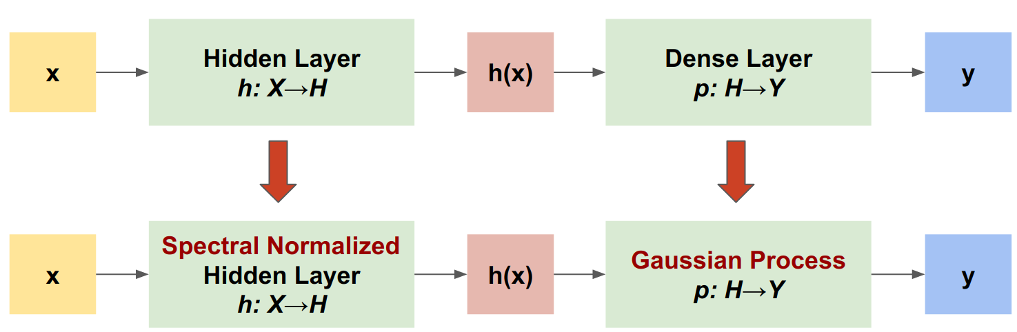
"SNGP 是一种可提高深度分类器的不确定性质量,同时能够保持相似准确率和延迟水平的简单方式。给定一个深度残差网络,SNGP 即会对模型进行两项简单更改:\n",
"\n",
"- 将谱归一化应用于隐藏的残差层。\n",
"- 将 Dense 输出层替换为高斯过程层。"
]
},
{
"cell_type": "markdown",
"metadata": {
"id": "ffU8rJ_eWHou"
},
"source": [
"> \n"
]
},
{
"cell_type": "markdown",
"metadata": {
"id": "2L88PoKr6XaE"
},
"source": [
"与其他不确定性方式(例如蒙特卡罗随机失活或深度集成)相比,SNGP 具有以下几项优点:\n",
"\n",
"- 适用于各种最先进的基于残差的架构(例如 (Wide) ResNet、DenseNet 或 BERT)。\n",
"- 是一种单模型方法(不依赖于集合平均)。因此,SNGP 具有与单一确定性网络相似的延迟水平,并且可以轻松扩展至大型数据集,如 [ImageNet](https://github.com/google/uncertainty-baselines/tree/main/baselines/imagenet){.external} 和 [Jigsaw 恶意评论分类](https://github.com/google/uncertainty-baselines/tree/main/baselines/toxic_comments){.external}。\n",
"- *距离感知*属性使之具有强大的域外检测性能。\n",
"\n",
"这种方法的缺点为:\n",
"\n",
"- SNGP 的预测不确定性是使用[拉普拉斯近似](http://www.gaussianprocess.org/gpml/chapters/RW3.pdf){.external}计算的。因此在理论上,SNGP 的后验不确定性与精确高斯过程的后验不确定性不同。\n",
"\n",
"- SNGP 训练需要在新周期开始时进行协方差重置步骤。这会对训练流水线额外增添些许复杂性。本教程展示了一种使用 Keras 回调实现此功能的简单方式。"
]
},
{
"cell_type": "markdown",
"metadata": {
"id": "ck_O7S8r1boS"
},
"source": [
"## 安装"
]
},
{
"cell_type": "code",
"execution_count": null,
"metadata": {
"id": "MOS9qFlW2o3J"
},
"outputs": [],
"source": [
"!pip install -U -q --use-deprecated=legacy-resolver tf-models-official tensorflow"
]
},
{
"cell_type": "code",
"execution_count": null,
"metadata": {
"id": "RCoGSYz-PIR7"
},
"outputs": [],
"source": [
"# refresh pkg_resources so it takes the changes into account.\n",
"import pkg_resources\n",
"import importlib\n",
"importlib.reload(pkg_resources)"
]
},
{
"cell_type": "code",
"execution_count": null,
"metadata": {
"id": "nJKtMbtYNXHn"
},
"outputs": [],
"source": [
"import matplotlib.pyplot as plt\n",
"import matplotlib.colors as colors\n",
"\n",
"import sklearn.datasets\n",
"\n",
"import numpy as np\n",
"import tensorflow as tf\n",
"\n",
"import official.nlp.modeling.layers as nlp_layers"
]
},
{
"cell_type": "markdown",
"metadata": {
"id": "8RCyTrQO4ZXo"
},
"source": [
"定义呈现宏"
]
},
{
"cell_type": "code",
"execution_count": null,
"metadata": {
"id": "o5VTrcxo3rI-"
},
"outputs": [],
"source": [
"plt.rcParams['figure.dpi'] = 140\n",
"\n",
"DEFAULT_X_RANGE = (-3.5, 3.5)\n",
"DEFAULT_Y_RANGE = (-2.5, 2.5)\n",
"DEFAULT_CMAP = colors.ListedColormap([\"#377eb8\", \"#ff7f00\"])\n",
"DEFAULT_NORM = colors.Normalize(vmin=0, vmax=1,)\n",
"DEFAULT_N_GRID = 100"
]
},
{
"cell_type": "markdown",
"metadata": {
"id": "lL5HzdYT5x5J"
},
"source": [
"## 双月数据集"
]
},
{
"cell_type": "markdown",
"metadata": {
"id": "nqazrSzhd24R"
},
"source": [
"从 [scikit-learn 双月数据集](https://scikit-learn.org/stable/modules/generated/sklearn.datasets.make_moons.html){.external} 创建训练数据集和评估数据集。"
]
},
{
"cell_type": "code",
"execution_count": null,
"metadata": {
"id": "xJ_ul9Ii52mh"
},
"outputs": [],
"source": [
"def make_training_data(sample_size=500):\n",
" \"\"\"Create two moon training dataset.\"\"\"\n",
" train_examples, train_labels = sklearn.datasets.make_moons(\n",
" n_samples=2 * sample_size, noise=0.1)\n",
"\n",
" # Adjust data position slightly.\n",
" train_examples[train_labels == 0] += [-0.1, 0.2]\n",
" train_examples[train_labels == 1] += [0.1, -0.2]\n",
"\n",
" return train_examples, train_labels"
]
},
{
"cell_type": "markdown",
"metadata": {
"id": "goQkrxR_fFGd"
},
"source": [
"评估模型在整个二维输入空间上的预测行为。"
]
},
{
"cell_type": "code",
"execution_count": null,
"metadata": {
"id": "Cj7ldkNw5-cT"
},
"outputs": [],
"source": [
"def make_testing_data(x_range=DEFAULT_X_RANGE, y_range=DEFAULT_Y_RANGE, n_grid=DEFAULT_N_GRID):\n",
" \"\"\"Create a mesh grid in 2D space.\"\"\"\n",
" # testing data (mesh grid over data space)\n",
" x = np.linspace(x_range[0], x_range[1], n_grid)\n",
" y = np.linspace(y_range[0], y_range[1], n_grid)\n",
" xv, yv = np.meshgrid(x, y)\n",
" return np.stack([xv.flatten(), yv.flatten()], axis=-1)"
]
},
{
"cell_type": "markdown",
"metadata": {
"id": "G9BYe4yqfeFa"
},
"source": [
"要评估模型不确定性,请添加属于第三类的域外 (OOD) 数据集。该模型在训练期间从不观测这些 OOD 样本。"
]
},
{
"cell_type": "code",
"execution_count": null,
"metadata": {
"id": "5UHz2SU4feSI"
},
"outputs": [],
"source": [
"def make_ood_data(sample_size=500, means=(2.5, -1.75), vars=(0.01, 0.01)):\n",
" return np.random.multivariate_normal(\n",
" means, cov=np.diag(vars), size=sample_size)"
]
},
{
"cell_type": "code",
"execution_count": null,
"metadata": {
"id": "l1-jmJb45_at"
},
"outputs": [],
"source": [
"# Load the train, test and OOD datasets.\n",
"train_examples, train_labels = make_training_data(\n",
" sample_size=500)\n",
"test_examples = make_testing_data()\n",
"ood_examples = make_ood_data(sample_size=500)\n",
"\n",
"# Visualize\n",
"pos_examples = train_examples[train_labels == 0]\n",
"neg_examples = train_examples[train_labels == 1]\n",
"\n",
"plt.figure(figsize=(7, 5.5))\n",
"\n",
"plt.scatter(pos_examples[:, 0], pos_examples[:, 1], c=\"#377eb8\", alpha=0.5)\n",
"plt.scatter(neg_examples[:, 0], neg_examples[:, 1], c=\"#ff7f00\", alpha=0.5)\n",
"plt.scatter(ood_examples[:, 0], ood_examples[:, 1], c=\"red\", alpha=0.1)\n",
"\n",
"plt.legend([\"Positive\", \"Negative\", \"Out-of-Domain\"])\n",
"\n",
"plt.ylim(DEFAULT_Y_RANGE)\n",
"plt.xlim(DEFAULT_X_RANGE)\n",
"\n",
"plt.show()"
]
},
{
"cell_type": "markdown",
"metadata": {
"id": "nlzxsnBBkybB"
},
"source": [
"这里,蓝色和橙色代表正负类,红色代表 OOD 数据。能够准确量化不确定性的模型在接近训练数据时(即 $p(x_{test})$ 接近 0 或 1)应达到较高的置信度,而在远离训练数据区域时(即 $p(x_{test})$ 接近 0.5)则不确定性较高。"
]
},
{
"cell_type": "markdown",
"metadata": {
"id": "RJ3i4n8li-Mv"
},
"source": [
"## 确定性模型"
]
},
{
"cell_type": "markdown",
"metadata": {
"id": "Utncgxs3lc4u"
},
"source": [
"### 定义模型"
]
},
{
"cell_type": "markdown",
"metadata": {
"id": "-z83-nq6jPlb"
},
"source": [
"从(基线)确定性模型开始:具有随机失活正则化的多层残差网络 (ResNet)。"
]
},
{
"cell_type": "code",
"execution_count": null,
"metadata": {
"cellView": "form",
"id": "wCBRm8fc6CgY"
},
"outputs": [],
"source": [
"#@title\n",
"class DeepResNet(tf.keras.Model):\n",
" \"\"\"Defines a multi-layer residual network.\"\"\"\n",
" def __init__(self, num_classes, num_layers=3, num_hidden=128,\n",
" dropout_rate=0.1, **classifier_kwargs):\n",
" super().__init__()\n",
" # Defines class meta data.\n",
" self.num_hidden = num_hidden\n",
" self.num_layers = num_layers\n",
" self.dropout_rate = dropout_rate\n",
" self.classifier_kwargs = classifier_kwargs\n",
"\n",
" # Defines the hidden layers.\n",
" self.input_layer = tf.keras.layers.Dense(self.num_hidden, trainable=False)\n",
" self.dense_layers = [self.make_dense_layer() for _ in range(num_layers)]\n",
"\n",
" # Defines the output layer.\n",
" self.classifier = self.make_output_layer(num_classes)\n",
"\n",
" def call(self, inputs):\n",
" # Projects the 2d input data to high dimension.\n",
" hidden = self.input_layer(inputs)\n",
"\n",
" # Computes the ResNet hidden representations.\n",
" for i in range(self.num_layers):\n",
" resid = self.dense_layers[i](hidden)\n",
" resid = tf.keras.layers.Dropout(self.dropout_rate)(resid)\n",
" hidden += resid\n",
"\n",
" return self.classifier(hidden)\n",
"\n",
" def make_dense_layer(self):\n",
" \"\"\"Uses the Dense layer as the hidden layer.\"\"\"\n",
" return tf.keras.layers.Dense(self.num_hidden, activation=\"relu\")\n",
"\n",
" def make_output_layer(self, num_classes):\n",
" \"\"\"Uses the Dense layer as the output layer.\"\"\"\n",
" return tf.keras.layers.Dense(\n",
" num_classes, **self.classifier_kwargs)"
]
},
{
"cell_type": "markdown",
"metadata": {
"id": "4u870GAen2aO"
},
"source": [
"本教程使用具有 128 个隐藏单元的六层 ResNet。"
]
},
{
"cell_type": "code",
"execution_count": null,
"metadata": {
"id": "bWL9wCnGpc4h"
},
"outputs": [],
"source": [
"resnet_config = dict(num_classes=2, num_layers=6, num_hidden=128)"
]
},
{
"cell_type": "code",
"execution_count": null,
"metadata": {
"id": "I47RY26wurgg"
},
"outputs": [],
"source": [
"resnet_model = DeepResNet(**resnet_config)"
]
},
{
"cell_type": "code",
"execution_count": null,
"metadata": {
"id": "okQXf2F1ur16"
},
"outputs": [],
"source": [
"resnet_model.build((None, 2))\n",
"resnet_model.summary()"
]
},
{
"cell_type": "markdown",
"metadata": {
"id": "8ZzueLoImW0t"
},
"source": [
"### 训练模型"
]
},
{
"cell_type": "markdown",
"metadata": {
"id": "JfQ1k-IUukLt"
},
"source": [
"配置训练参数以使用 `SparseCategoricalCrossentropy` 作为损失函数和 Adam 优化器。"
]
},
{
"cell_type": "code",
"execution_count": null,
"metadata": {
"id": "a9ZkfNXAnumV"
},
"outputs": [],
"source": [
"loss = tf.keras.losses.SparseCategoricalCrossentropy(from_logits=True)\n",
"metrics = tf.keras.metrics.SparseCategoricalAccuracy(),\n",
"optimizer = tf.keras.optimizers.legacy.Adam(learning_rate=1e-4)\n",
"\n",
"train_config = dict(loss=loss, metrics=metrics, optimizer=optimizer)"
]
},
{
"cell_type": "markdown",
"metadata": {
"id": "wEWzfHvf6A5_"
},
"source": [
"以 128 为批次大小对模型训练 100 个周期。"
]
},
{
"cell_type": "code",
"execution_count": null,
"metadata": {
"id": "1Fx6EtGXpzVr"
},
"outputs": [],
"source": [
"fit_config = dict(batch_size=128, epochs=100)"
]
},
{
"cell_type": "code",
"execution_count": null,
"metadata": {
"id": "cFwkbKIuqj7Y"
},
"outputs": [],
"source": [
"resnet_model.compile(**train_config)\n",
"resnet_model.fit(train_examples, train_labels, **fit_config)"
]
},
{
"cell_type": "markdown",
"metadata": {
"id": "eo6tKKd1rvBh"
},
"source": [
"### 呈现不确定性"
]
},
{
"cell_type": "code",
"execution_count": null,
"metadata": {
"cellView": "form",
"id": "HZDMX7gZrZ-5"
},
"outputs": [],
"source": [
"#@title\n",
"def plot_uncertainty_surface(test_uncertainty, ax, cmap=None):\n",
" \"\"\"Visualizes the 2D uncertainty surface.\n",
" \n",
" For simplicity, assume these objects already exist in the memory:\n",
"\n",
" test_examples: Array of test examples, shape (num_test, 2).\n",
" train_labels: Array of train labels, shape (num_train, ).\n",
" train_examples: Array of train examples, shape (num_train, 2).\n",
" \n",
" Arguments:\n",
" test_uncertainty: Array of uncertainty scores, shape (num_test,).\n",
" ax: A matplotlib Axes object that specifies a matplotlib figure.\n",
" cmap: A matplotlib colormap object specifying the palette of the\n",
" predictive surface.\n",
"\n",
" Returns:\n",
" pcm: A matplotlib PathCollection object that contains the palette\n",
" information of the uncertainty plot.\n",
" \"\"\"\n",
" # Normalize uncertainty for better visualization.\n",
" test_uncertainty = test_uncertainty / np.max(test_uncertainty)\n",
"\n",
" # Set view limits.\n",
" ax.set_ylim(DEFAULT_Y_RANGE)\n",
" ax.set_xlim(DEFAULT_X_RANGE)\n",
"\n",
" # Plot normalized uncertainty surface.\n",
" pcm = ax.imshow(\n",
" np.reshape(test_uncertainty, [DEFAULT_N_GRID, DEFAULT_N_GRID]),\n",
" cmap=cmap,\n",
" origin=\"lower\",\n",
" extent=DEFAULT_X_RANGE + DEFAULT_Y_RANGE,\n",
" vmin=DEFAULT_NORM.vmin,\n",
" vmax=DEFAULT_NORM.vmax,\n",
" interpolation='bicubic',\n",
" aspect='auto')\n",
"\n",
" # Plot training data.\n",
" ax.scatter(train_examples[:, 0], train_examples[:, 1],\n",
" c=train_labels, cmap=DEFAULT_CMAP, alpha=0.5)\n",
" ax.scatter(ood_examples[:, 0], ood_examples[:, 1], c=\"red\", alpha=0.1)\n",
"\n",
" return pcm"
]
},
{
"cell_type": "markdown",
"metadata": {
"id": "a1age2y0339T"
},
"source": [
"现在,呈现确定性模型的预测。首先绘制类概率:$$p(x) = softmax(logit(x))$$"
]
},
{
"cell_type": "code",
"execution_count": null,
"metadata": {
"id": "4aqFgQOD40lb"
},
"outputs": [],
"source": [
"resnet_logits = resnet_model(test_examples)\n",
"resnet_probs = tf.nn.softmax(resnet_logits, axis=-1)[:, 0] # Take the probability for class 0."
]
},
{
"cell_type": "code",
"execution_count": null,
"metadata": {
"id": "rpflH2Qj33oN"
},
"outputs": [],
"source": [
"_, ax = plt.subplots(figsize=(7, 5.5))\n",
"\n",
"pcm = plot_uncertainty_surface(resnet_probs, ax=ax)\n",
"\n",
"plt.colorbar(pcm, ax=ax)\n",
"plt.title(\"Class Probability, Deterministic Model\")\n",
"\n",
"plt.show()"
]
},
{
"cell_type": "markdown",
"metadata": {
"id": "7ShGAB7FNYgU"
},
"source": [
"在此图中,黄色和紫色为这两个类的预测概率。确定性模型在利用非线性决策边界对两个已知类(蓝色和橙色)进行分类方面表现优秀。然而,它并不具备**距离感知**,并且会以较高的置信度将从未观测到的红色域外 (OOD) 样本分类为橙色类。\n",
"\n",
"通过计算[预测方差](https://en.wikipedia.org/wiki/Bernoulli_distribution#Variance)来呈现模型的不确定性:$$var(x) = p(x) * (1 - p(x))$$ 在 GitHub 上查看源代码