Intro

Welcome to Practical Observability, an online mdbook powered book that covers topics around observability in modern software systems specifically using the Prometheus metrics model and OpenTelemetry's distributed tracing model.

Observability

In control theory, observability (o11y) is defined as a measure of how well internal states of a system can be inferred from knowledge of its external outputs.¹

For software systems, observability is a measure of how well you can understand and explain any state your system can get into.¹

Observability has three traditionally agreed-upon pillars and a fourth more emergent pillar: Metrics, Logging, Tracing, and Profiling.

This book aims to provide a primer on each of these pillars of o11y through the lens of a common open source observability tooling vendor, Grafana.

Through the sections of this chapter, you will be able to learn the fundamentals of Metrics, Logging, Tracing, and Profiling, see code samples in two popular coding languages (Python and Golang), and develop the skills required to create high signal, insightful dashboards to increase visibility and reduce Mean Time to Resolution for production incidents.

Lots of content for these docs is inspired and sometimes directly drawn from Charity Majors, Liz Fong-Jones, and George Miranda's book, "Observability Engineering"

Metrics

What Metrics are Not

Metrics are not a silver bullet to solving all your production issues. In fact, in a world of microservices where each service talks to a number of other services in order to serve a request, metrics can be deceptive, difficult to understand, and are often missing where we need them most because we failed to anticipate what we should have been measuring.

In a modern world, debugging with metrics requires you to connect dozens of disconnected metrics that were recorded over the course of executing any one particular request, across any number of services or machines, to infer what might have occurred over the various hops needed for its fulfillment. The helpfulness of those dozens of clues depends entirely upon whether someone was able to predict, in advance, if that measurement was over or under the threshold that meant this action contributed to creating a previously unknown anomalous failure mode that had never been previously encountered.¹

That being said, metrics can be useful in the process of debugging and triaging production incidents. Metrics provide a helpful summary of the state of a system, and while they may not hold all the answers, they allow us to ask more specific questions which help to guide investigations. Additionally, metrics can be the basis for alerts which provide on-call engineers with early warnings, helping us catch incidents before they impact users.

What Metrics Are

Metrics are numerical time-series data that describe the state of systems over time.

Common base metrics include the following:

Latency between receiving a HTTP request and sending a response
CPU seconds being utilized by a system
Number of requests being processed by a system
Size of response bodies being sent by a system
Number of requests that result in errors being sent by a system

These base metrics are all things we can measure directly in a given system. They don't immediately seem useful in determining if something is wrong with the system but from these core metrics we can derive higher level metrics that indicate when systems may be unhealthy.

Common derived metrics include:

95th Percentile of HTTP Request/Response Latency over the past 5 minutes
Average and Maximum CPU Utilization % across all deployed containers for a system over the past hour
Request throughput ($ \frac{req}{s}$) being handled by a system over the past 5 minutes
Ingress and Egress Bandwidth ($ \frac{MB}{s}$) of a system over the past hour
Error ($\frac{failed\ requests}{total\ requests}$) rate ($ \frac{error}{s}$) of a system over the past 5 minutes

Derived metrics, when graphed, make it easy to visually pattern match to find outliers in system operation. Derived metrics can also be utilized for alerting when outside of "normal" operating ranges, but generally don't determine directly that there is something wrong with the system.

As engineers, we track base metrics in our systems and expose them for collection regularly so that our observability platform can record the change over time of these base metrics. We pick base metrics that provide measurable truth of the state of the system using absolute values where possible. With a large enough pool of base metrics, we can generate dozens of derived metrics that interpret the base metrics in context, making it clear to the viewer both what is being measured and why it is important.

Lots of content for these docs is inspired and sometimes directly drawn from Charity Majors, Liz Fong-Jones, and George Miranda's book, "Observability Engineering"

Labels

In most metrics systems, metrics are stored as multi-dimensional time series where the primary dimension is the observed value at a given time.

Labels are additional categorical dimensions for a metric that allow you to differentiate observations by some property.

Example of labels for metrics are as follows:

Metric	Label
CPU Utilization of a system	Kubernetes Pod Name for each instance of the system
Latency of handling an HTTP Request	Status code of the HTTP response
Number of requests served by a service	Path requested by the user (not including parameters)

Label Cardinality

Each metric can have any number of Labels, but for each unique value of a Label, your metrics system will need to create and maintain a whole new time series to track the Label-specific dimension of the metric.

Given the example label of Status code of the HTTP response, if our initial metric is a simple time series like Number of requests served by a service, then by adding the status code Label, we're potentially creating hundreds of new time series to track our metric, one for each HTTP Status Code that can be reported by our system. Let's say that our service only uses 20 HTTP response codes, that label gets us to 20 time series (one per unique label value) since our original metric is a Counter that only requires one initial time series to track.

When adding a second label like Kubernetes Pod Name for each instance of the system, we aren't adding one new time series for each Pod Name but are multiplying our existing time series by the number of unique values for this new label. In this case, if we have 10 pods each running an instance of our service, we'll end up with 1 * 20 * 10 = 200 time series for our metric.

You can see how a metric with 8 labels each with 5 unique values can quickly add up, and adding just one extra label to a metric with many existing labels quickly becomes unsustainable:

\[ 1*5^{8} = 32{,}768 \]

\[ 1*5^{9} = 1{,}953{,}125\]

The uniqueness of a label value can be described by the term cardinality where a high cardinality label would have many unique values and a low cardinality label would have few unique values.

An example high cardinality label could be something like IP Address of Requester for a web service with many unique users (cardinality equal to number of unique users).

An example low cardinality label could be something like HTTP Status Group (2xx,3xx,4xx,5xx) of Response for a web service (cardinality of 4).

Metric Dimensionality

The cost of a metric is generally proportional to its dimensionality where the dimensionality of a metric is the total number of time series required to keep track of the metric and its labels.

In our example above, our Number of requests served by a service metric has a dimensionality of 1 * 20 * 10 = 200 meaning we need 200 time series in our metric system to track the metric. If we changed the Status code of the HTTP response label to be a HTTP Status Group (2xx,3xx,4xx,5xx) of Response label, our dimensionality would reduce to 1 * 4 * 10 = 40 time series which significantly reduces the cost of tracking this metric.

Higher Dimensionality metrics provide more detail and help answer more specific questions, but they do so at the cost of maintaining significantly more time series (which each have an ongoing storage and processing cost). Save High Dimensionality metrics for the things that really need a high level of detail, while picking low cardinality Labels for generic metrics to keep dimensionality low. There are always tradeoffs in observability between cost and detail and Metric Dimensionality is one of the best examples of such a tradeoff.

Metric Types

This section will draw heavily from the Prometheus Docs and more can be explored there but frankly they don't go super into depth into the mechanics of metric types and do a poor job of consolidating what you need to know.

Prometheus's metrics client libraries usually expose metrics for a service at an HTTP endpoint like /metrics.

If you visit this endpoint, you will see a newline separated list of metrics like the one below with an optional HELP directive describing the metric, a TYPE directive describing the Metric Type, and one or more lines of Values for the metric that reflect the immediate values for the given metric.

# HELP process_cpu_seconds_total Total user and system CPU time spent in seconds.
# TYPE process_cpu_seconds_total counter
process_cpu_seconds_total 693.63

# HELP process_open_fds Number of open file descriptors.
# TYPE process_open_fds gauge
process_open_fds 16

# HELP api_response_time Latency of handling an HTTP Request
# TYPE api_response_time histogram
api_response_time_bucket{le="0.005"} 1.887875e+06
api_response_time_bucket{le="0.01"} 1.953018e+06
api_response_time_bucket{le="0.025"} 1.979542e+06
api_response_time_bucket{le="0.05"} 1.985364e+06
api_response_time_bucket{le="0.1"} 1.98599e+06
api_response_time_bucket{le="0.25"} 1.986053e+06
api_response_time_bucket{le="0.5"} 1.986076e+06
api_response_time_bucket{le="1"} 1.986084e+06
api_response_time_bucket{le="2.5"} 1.986087e+06
api_response_time_bucket{le="5"} 1.986087e+06
api_response_time_bucket{le="10"} 1.986087e+06
api_response_time_bucket{le="+Inf"} 1.986087e+06
api_response_time_sum 3930.0361077078646
api_response_time_count 1.986087e+06

# HELP go_gc_duration_seconds A summary of the pause duration of garbage collection cycles.
# TYPE go_gc_duration_seconds summary
go_gc_duration_seconds{quantile="0"} 0.000130274
go_gc_duration_seconds{quantile="0.25"} 0.000147971
go_gc_duration_seconds{quantile="0.5"} 0.000155235
go_gc_duration_seconds{quantile="0.75"} 0.000168787
go_gc_duration_seconds{quantile="1"} 0.000272923
go_gc_duration_seconds_sum 0.298708187
go_gc_duration_seconds_count 1815

The Prometheus model uses Scraping by default, where some Agent will poll the /metrics endpoint every n seconds (usually 60 seconds) and record discrete values for every time series described by the endpoint. Because this polling is not continuous, when a metric is updated in your service, it may not create a discrete datapoint until the next time Scraper comes by. This is an optimization that reduces the amount of work needed to be done by both your service and the Scraper, but if you need to create datapoints synchronously (like for a batch job that exits after it finishes whether or not a Scraper has a chance to poll its /metrics endpoint), Prometheus has a Push Gateway pattern. We will dive deeper into Pushing Metrics later in this chapter.

Counters

The fundamental metric type (at least in Prometheus's metrics model) is a Counter. A Counter is a monotonically increasing (only counts up), floating point value that starts at 0 when initialized.

It's important to note that when an application starts up, all of its metrics are initialized to zero and instrumentation libraries cumulatively build on this zero value through the lifetime of the application. You may have a container with a service in it that's been running for two months where a Counter has incremented itself to 1,525,783 but as soon as the container restarts that Counter will read as 0.

Counters are useful metrics for tracking a number of times something has happened since the start of the service. Some examples of things you might track with a counter include:

Number of requests handled
Number of calls to an external service
Number of responses with a particular status code
Number of errors in processing requests
Number of jobs executed

In our example payload, the Counter metric is represented as follows:

# HELP process_cpu_seconds_total Total user and system CPU time spent in seconds.
# TYPE process_cpu_seconds_total counter
process_cpu_seconds_total 693.63

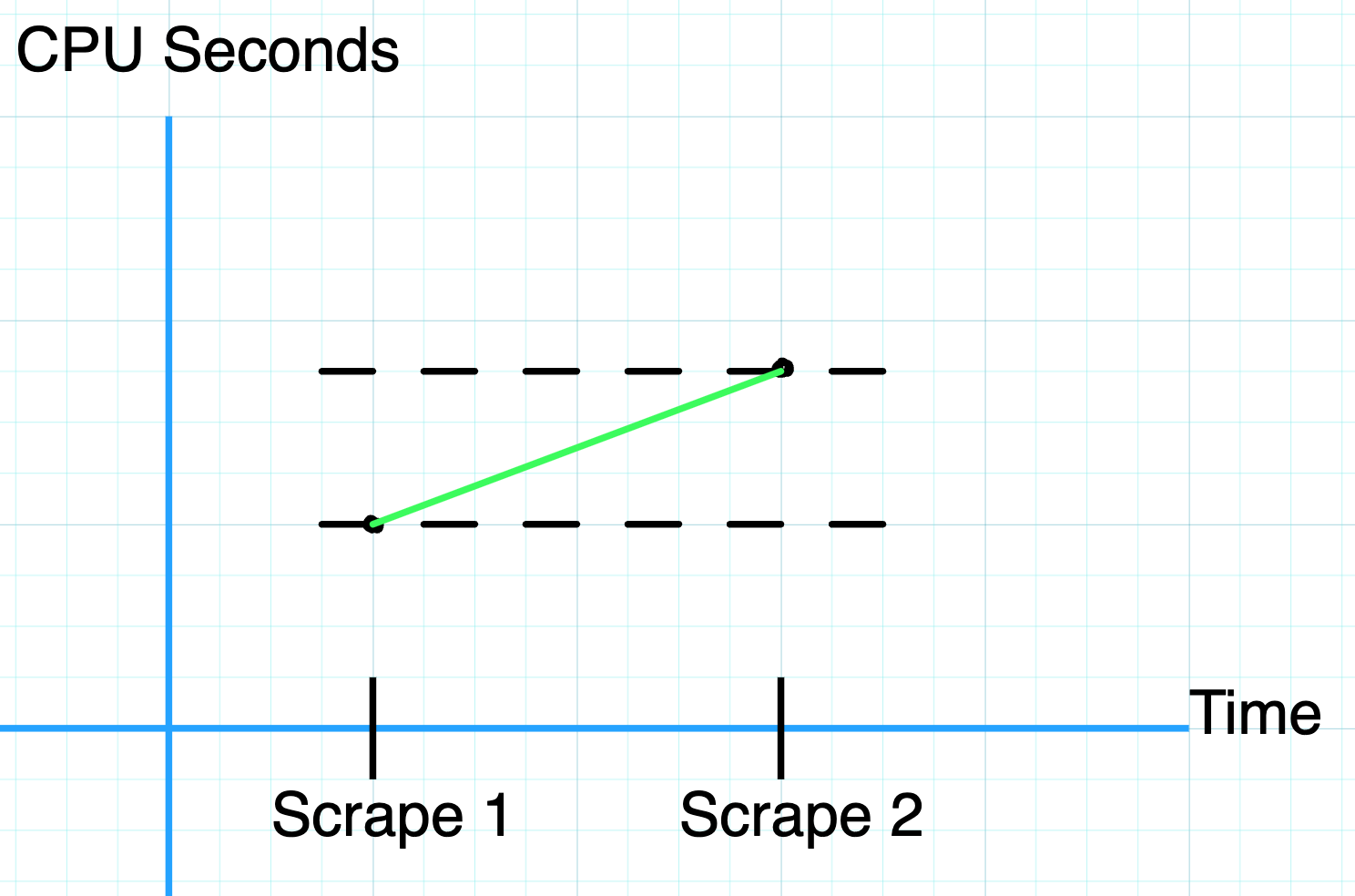
This metric tracks the CPU time consumed by our service. It starts at 0 when the service starts and slowly climbs over time. This number will increase forever if our service never restarts. Prometheus's Counter implementation handles that by representing numbers in E Notation once they get large enough. For example, 1.986087e+06 is equivalent to $1.986087 * 10^{6} = 1{,}986{,}087$. Clearly, as we represent larger and larger numbers in our metrics, we lose precision, but generally the larger the numbers we are tracking, the larger the changes are and the less precision we need to identify patterns in the system.

Because counters are monotonically increasing values, even though scrape intervals may be minutes apart, we can interpolate the values in between to decent accuracy. In the image below, we know the values between Scrape 1 and Scrape 2 must be somewhere between the dotted lines, so we can estimate them as a straight line if we need to guess at the value in between scrapes.

Counter Interpolation Graph

Querying Counter Metrics

To explore Counter metrics, let's build a Prometheus query in PromQL, Prometheus's Query Language.

To start, we can query our Prometheus instance for our counter metric by name: process_cpu_seconds_total.

A screenshot of the Prometheus Web UI searching for "process_cpu_seconds_total"

We can see that this given Prometheus instance has eight series being returned, with each series in the form:

process_cpu_seconds_total{instance="<some_address>", job="<some_job_name>"}

Prometheus represents metrics in PromQL using the following format:

<metric_name>{<label_1_key>="<label_1_value>", <label_2_key>="<label_2_value>", ..., <label_n_key>="<label_n_value>"}

In our example, we see two different labels, instance and job. The instance label has eight distinct values, as does the job label. Prometheus generates a new time series for each unique set of label values it encounters, so while the theoretical dimensionality of this metric may be 1 * 8 * 8 = 64, in practice there are only eight series being maintained.

Let's select one of these series to explore further.

In PromQL we can narrow the time series returned by our query by specifying filters for labels. The example below restricts the above results to only include those series where the instance label has a value that starts with localhost. To do this we use the =~ operator on the instance label to filter by a regex that matches anything starting with localhost.

process_cpu_seconds_total{instance=~"localhost.*"}

$A screenshot of the Prometheus Web UI searching for "process_cpu_seconds_total{instance=~"localhost.*"}"$

We can further filter by job to end up with a single series trivially using the = operator. Let's filter for the prometheus job using the following query:

process_cpu_seconds_total{instance=~"localhost.*", job="prometheus"}

Note that we could technically have just used the job query here since there is only one series with a job label with value prometheus.

$A screenshot of the Prometheus Web UI searching for "process_cpu_seconds_total{instance=~"localhost.*", job="prometheus"}"$

From here, we can click on the Graph tab to view our metric in Prometheus's built-in graphing tool, though we'll go over building more interesting graphs in Grafana later.

$A screenshot of the Prometheus Web UI graphing "process_cpu_seconds_total{instance=~"localhost.*", job="prometheus"}" with a 1 hour window$

As this is a Counter metric, we expect to see a monotonically increasing graph, which is quite clear, but why does the line look perfectly smooth if we didn't do anything to interpolate values? If we set the time range to something smaller than an hour, such as five minutes, the graph starts to look a bit different.

$A screenshot of the Prometheus Web UI graphing "process_cpu_seconds_total{instance=~"localhost.*", job="prometheus"}" with a 5 minute window$

Now we can see the bumpiness we would expect of many discrete observations spaced an equal amount of time apart.

An even more intense zoom reveals the gap between observations to be five seconds for our given metric. Each stair step has a length of four seconds and then the line up to the next stair has a length of one second meaning our observations are separated by a total of five seconds.

$A screenshot of the Prometheus Web UI graphing "process_cpu_seconds_total{instance=~"localhost.*", job="prometheus"}" with a 10 second window$

Range Vectors and the Rate Query

While this graph is neat, it doesn't exactly make much sense as a raw series. Total CPU Seconds used by a service is interesting but it would be much more useful to see it as a rate of CPU usage in a format like CPU Seconds per Second. Thankfully, PromQL can help us derive a rate from this metric as follows:

rate(process_cpu_seconds_total{instance=~"localhost.*", job="prometheus"}[1m])

In this query we're making use of the rate() Query Function in PromQL which calculates the "per-second average rate of increase in the time series in the range vector". This is effectively the slope of the line of the raw observed value with a bit of added nuance. To break that down a bit, the "range vector" in our query is [1m], meaning for each observation, we are grabbing the value of the metric at that time, then the values of previous observations for that metric from one minute prior to the selected observation. Once we have that list of values, we calculate the rate of increase between each successive observation, then average it out over the one minute period. For a monotonically increasing Counter value, we can simplify the equation by grabbing the first and last points in our range vector, grabbing the difference in values and dividing by the time between the two observations. Let's show it the hard way and then we can simplify.

Consider the following observations for a given counter metric, requests, in the form [time, counter_value]:

[0, 0], [10, 4], [20, 23], [30, 31], [40, 45], [50, 63], [60, 74], [70, 102]

If we wanted to take the rate(requests{}[30s]) at the point [40, 45] we would grab 30 seconds worth of observations, so all those going back to [10, 4]. Then we calculate the increase between each successive observation:

[10, 4] to [20, 23] -> 23 - 4 = 19
[20, 23] to [30, 31] -> 31 - 23 = 8
[30, 31] to [40, 45] -> 45 - 31 = 14

Since our observations are evenly spaced, we can average the per-second rate of increase as: \[ \frac{19}{10} + \frac{8}{10} + \frac{14}{10} = 1.\overline{33}\]

As we're using a Counter, we can simplify the process by grabbing the first and last observations in the range and calculating the difference between them and divide by the number of seconds between the observations: \[ \frac{45-4}{30} = 1.\overline{33}\]

That only gives us the rate(requests{}[30s]) at the time=40 point, but that process is repeated for every observation visible at the resolution we're requesting.

The result of this operation on our process_cpu_seconds_total metric is graphed below:

$A screenshot of the Prometheus Web UI graphing "rate(process_cpu_seconds_total{instance=~"localhost.*", job="prometheus"}[1m])" with a 1 hour window$

From this graph we can see that in the past hour our service peaks its usage at a little over 0.04 CPU Seconds per Second or around 4% of a single CPU core.

Gauges

The second metric type we need to know about is a Gauge.

Gauges are very similar to Counters in that they are a floating point value that starts initialized to zero, however a Gauge can go both up and down and has the potential to be either a positive or negative number.

Gauges are useful metrics for tracking a specific internal state value that fluctuates up and down throughout service lifetime:

Temperature of a sensor
Bytes of memory currently allocated
Number of pending requests in the queue
Number of active routines
Number of active TCP connections
Number of open File Descriptors

In our example payload, the Gauge metric is represented as follows:

# HELP process_open_fds Number of open file descriptors.
# TYPE process_open_fds gauge
process_open_fds 16

Gauges are useful to interrogate the immediate internal state of a service at a given point in time.

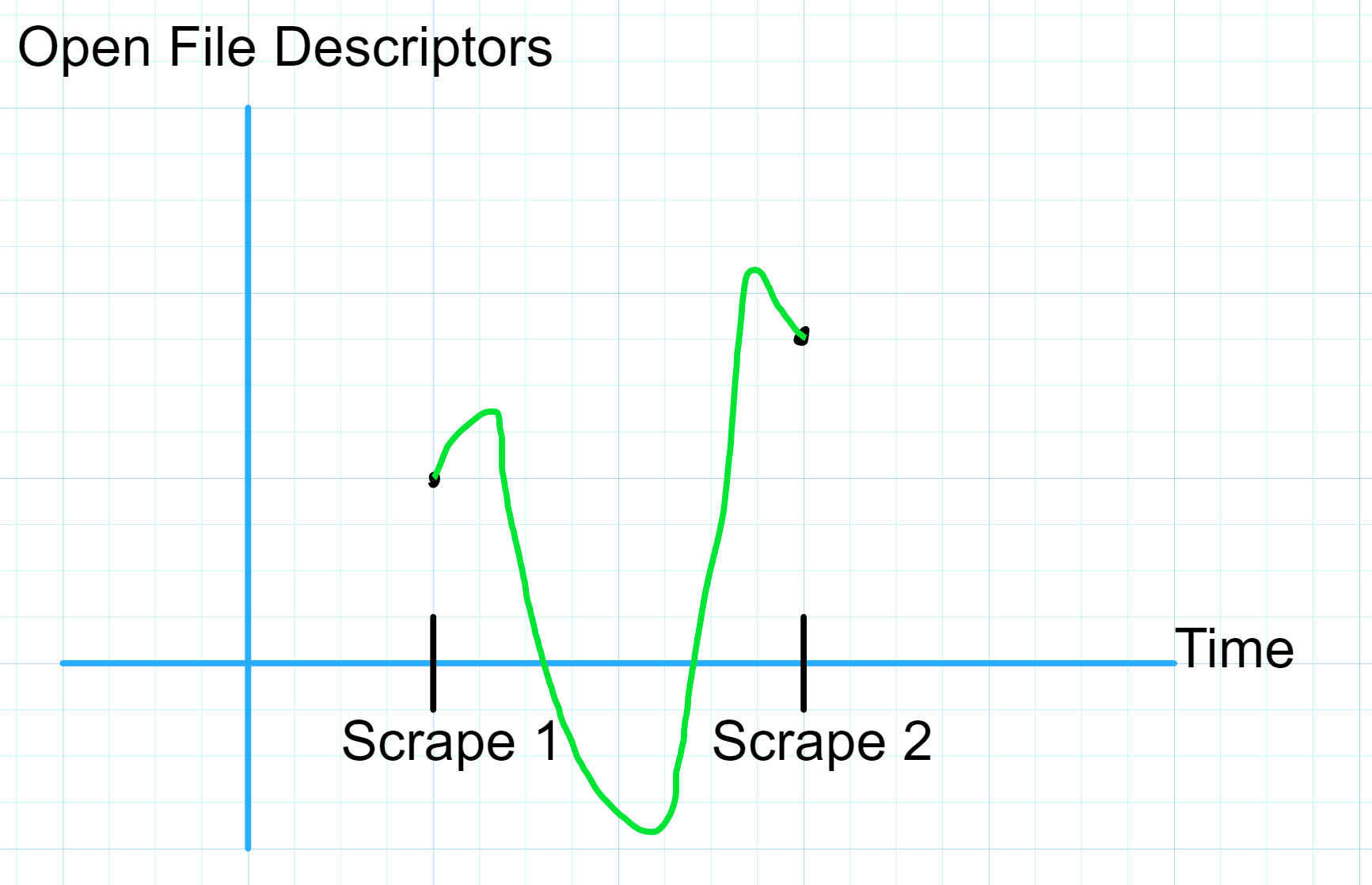
Unlike with Counters, calculating the rate() of a Gauge doesn't really make sense since Gauge values can go up and down between observations.

We are unable to interpolate between two observations of a Gauge since we don't know the boundaries of possible values for the Gauge between the observations.

Graph of a Gauge with its true value wandering above and below both observed values in between them

In the absence of a rate() style query, how can we contextualize a Gauge metric?

Prometheus provides us with additional Range Vector functions to help interpret the values of Gauges by aggregating observations over time.

In the previous chapter on Counters, I introduce a concept of a Range Vector and walk through how the rate() query operates on such vectors. We'll be using Range Vectors below so feel free to go back and review if you need a refresher.

Below is a list of a few of the functions we can use to better understand what our Gauge is telling us about our service:

avg_over_time()
- Take all values in the range vector, add them up, and divide the sum by the number of observations in the vector.
min_over_time()
- Take the lowest value in the range vector (remember, Gauge values can be both positive or negative).
max_over_time()
- Take the highest value in the range vector.
sum_over_time()
- Take all values in the range vector and add them up.
quantile_over_time()
- Keep reading for a breakdown.

There are a few others available to us but for the purposes of this chapter we'll explore the above five functions in a practical scenario.

The Quantile Function

The Quantile Function is a commonly used function in probability theory and statistics but I am neither a statistician or probabilist.

Thankfully we don't need probability theory to understand what quantile_over_time() does and how it works.

Given a Range Vector (list of successive observations of a Gauge) vec and a target Quantile of 0.90, quantile_over_time(0.90, vec) returns the value at the 90th percentile of all observations in vec.

Recall that the 50th percentile of a series of numbers, also called the median, is the member of the series at which half of the remaining numbers in the series fall below and the other half fall above.

For a sample series:

[25, 45, 34, 88, 76, 53, 91, 21, 53, 12, 6, 37, 97, 50]

We find the median by sorting the series least-to-greatest and picking the value in the middle, or in the case of a series of even length, we average the two middle-most numbers.

[6, 12, 21, 25, 34, 37, (45, 50), 53, 53, 76, 88, 91, 97]

\[ \frac{45 + 50}{2} = 47.5\]

So in this example our median is 47.5 which is the same as the 50th percentile of the series.

Okay, so what does that make the 90th percentile? Well the 90th percentile of a series is the value for which 90% of the numbers in the series fall below and 10% of the numbers in the series fall above.

So given our example series, how do we find the 90th percentile?

Well if we have an ordered series of numbers, we'd want to grab the value at position 0.9 * n where n is the number of values in the series, since that would split the series into two chunks, one with 90% of the values and one with 10% of the values. In our example series, we have 14 values, so we'd take the value at position 0.9 * 14 = 12.6.

Since our series has 14 numbers in it, it is impossible to find a value at which exactly 90% of the values fall below it and 10% fall above it (14 is not divisible by 10), so we can estimate the 90th percentile for our series by taking the weighted average of the values on either side of the split point.

[6, 12, 21, 25, 34, 37, 45, 50, 53, 53, 76, (88, 91), 97]

\[ (88 * (1-0.6)) + (91 * 0.6) = 89.8\]

Now that we've cleared that up, it should be easy to get the 75th percentile of our Range Vector (or any other percentile we need), just use quantile_over_time(0.75, vec).

If we look at the implementation of the quantile_over_time() function in the Prometheus source we see a fairly straightforward Go function that does the same process we just walked through:

// quantile calculates the given quantile of a vector of samples.
// ...
func quantile(q float64, values vectorByValueHeap) float64 {
	//...
	sort.Sort(values)

	n := float64(len(values))
	// When the quantile lies between two samples,
	// we use a weighted average of the two samples.
    // Multiplying by (n-1) because our vector starts at index 0 in code
	rank := q * (n - 1) 

	lowerIndex := math.Max(0, math.Floor(rank))
	upperIndex := math.Min(n-1, lowerIndex+1)

	weight := rank - math.Floor(rank)
	return values[int(lowerIndex)].V*(1-weight) + values[int(upperIndex)].V*weight
}

Querying Gauge Metrics

Now let's put these functions into practice and learn a bit about our example metric, process_open_fds.

TODO: write about querying Gauge metrics

Go Instrumentation

This chapter will cover the process of adding Prometheus-style metrics instrumentation to your new or existing Go application.

Some of the following examples will be particular to HTTP APIs, but I'll also include an example of instrumenting a batch-style process that exits after completion and a long-running service that may not expose a traditional HTTP API.

The Go Prometheus Library

Grafana provides a Prometheus metrics client for Golang that has remained remarkably stable over the past 8 years.

While the OpenTelemetry project is incubating a Metrics package to to implement their vendor-agnostic Metrics Data Model, as of this writing, the package is in the Alpha state and is not recommended for general use until it graduates into the Stable state because it will likely have several breaking interface revisions before then.

Several other metrics packages have emerged over this time that wrap existing metrics clients like go-kit's metrics package, but at the end of the day the Prometheus client has remained reliably stable and consistent for years and the formats and patterns it established have helped define what system metrics look like everywhere today.

The package documentation lives here and provides a basic starting example and a deeper dive into the full capabilities of the client library, but I'll provide in-depth examples in the following sections.

Instrumenting a Simple HTTP Service

Imagine you have a service in Golang that exposes some HTTP API routes and you're interested in tracking some metrics pertaining to these routes. Later we'll cover instrumenting more complex services and using instrumentation packages for common frameworks like Gin and Echo to add some baseline metrics to existing services without having to manually instrument our handlers.

Defining an Example Service

package main

import (
	"encoding/json"
	"net/http"
)

// User is a struct representing a user object
type User struct {
	ID   int    `json:"id"`
	Name string `json:"name"`
}

var users []User

func main() {
	http.HandleFunc("/users", handleUsers)
	http.ListenAndServe(":8080", nil)
}

func handleUsers(w http.ResponseWriter, r *http.Request) {
	switch r.Method {
	case "GET":
		// List all users
		json.NewEncoder(w).Encode(users)
	case "POST":
		// Create a new user
		var user User
		json.NewDecoder(r.Body).Decode(&user)
		users = append(users, user)
		json.NewEncoder(w).Encode(user)
	default:
		http.Error(
			w,
			http.StatusText(http.StatusMethodNotAllowed),
			http.StatusMethodNotAllowed,
		)
	}
}

This code defines a struct called User that represents a user object. It has two fields: ID and Name.

The main() function sets up an HTTP server that listens on port 8080 and registers a handler function for requests to the /users endpoint.

The handleUsers() function is the handler for requests to the /users endpoint. It uses a switch statement to handle different HTTP methods (GET, POST, etc.) differently.

For example, when a GET request is received, it simply encodes the list of users as JSON and writes it to the response. When a POST request is received, it decodes the request body as a User object, appends it to the list of users, and then encodes the User object as JSON and writes it to the response.

Instrumenting the Example Service

Metrics we may be interested in tracking include which routes are called in a time period, how many times they're called, how long they take to handle, and what status code they return.

An Aside on Collectors, Gatherers, and Registries

The Prometheus client library initializes one or more Metrics Registries which are then periodically Collected, Gathered, and Exposed generally via an HTTP route like /metrics for scraping via library-managed goroutines.

For our purposes, we can generally rely on the implicit Global Registry to register our metrics and use the promauto package to initialize our Collectors behind the scenes. If you are a power user that wants to dig deeper into building custom Metrics Registries, Collectors or Gatherers, you can take a deeper dive into the docs here.

We'll import three packages at the top of our file:

import (
        //...
        "github.com/prometheus/client_golang/prometheus"
        "github.com/prometheus/client_golang/prometheus/promauto"
        "github.com/prometheus/client_golang/prometheus/promhttp"
)

The prometheus package is our client library, promauto handles registries and collectors for us, and promhttp will let us export our metrics to a provided HTTP Handler function so that our metrics can be scraped from /metrics.

Registering Metrics and Scraping Handler

Now we can initialize a CounterVec to keep track of calls to our API routes and use some labels on the counter to differentiate between the HTTP Method being used (POST vs GET).

A CounterVec is a group of Counter metrics that may have different label values, if we just used a Counter we'd have to define a different metric for each distinct label value.

When initializing the CounterVec we provide the keys or names of the labels in advance for registration, while the label values can be defined dynamically in our application when recording a metric observation.

Let's initialize our reqCounter CounterVec above the main() function and use the promhttp library to expose our metrics on /metrics:

//...
var users []User

// Define the CounterVec to keep track of Total Number of Requests
// Also declare the labels names "method" and "path"
var reqCounter = promauto.NewCounterVec(prometheus.CounterOpts{
	Name: "userapi_requests_handled_total",
	Help: "The total number of handled requests",
}, []string{"method", "path"})

func main() {
    // Expose Prometheus Metrics on /metrics
    http.Handle("/metrics", promhttp.Handler())

    // Register API route handlers
	http.HandleFunc("/users", handleUsers)

    // Startup the HTTP server on port 8080
	http.ListenAndServe(":8080", nil)
}
//...

Recording Observations of Custom Metrics

Finally we'll want to update our handleUsers() function to increment the Counter with the proper labels when we get requests as follows:

//...
func handleUsers(w http.ResponseWriter, r *http.Request) {
	switch r.Method {
	case "GET":
		// Increment the count of /users GETs
		reqCounter.With(prometheus.Labels{"method": "GET", "path": "/users"}).Inc()
		// List all users
		json.NewEncoder(w).Encode(users)
	case "POST":
		// Increment the count of /users POSTs
		reqCounter.With(prometheus.Labels{"method": "POST", "path": "/users"}).Inc()
		// Create a new user
		var user User
		json.NewDecoder(r.Body).Decode(&user)
		users = append(users, user)
		json.NewEncoder(w).Encode(user)
	default:
		http.Error(
			w,
			http.StatusText(http.StatusMethodNotAllowed),
			http.StatusMethodNotAllowed,
		)
	}
}

Testing our Instrumentation

Let's test our results by running the server, hitting the endpoints a few times, then watching the /metrics endpoint to see how it changes:

go run main.go

In another tab we can use curl to talk to the server at http://localhost:8080

$ # GET our /users route
$ curl http://localhost:8080/users
> null

$ # Check the /metrics endpoint to see if our metric appears
$ curl http://localhost:8080/metrics
> ...
> # HELP userapi_requests_handled_total The total number of handled requests
> # TYPE userapi_requests_handled_total counter
> userapi_requests_handled_total{method="GET",path="/users"} 1

Note that we see a single time series under the userapi_requests_handled_total heading with the label values specified in our GET handler.

$ # POST a new user and then fetch it
$ curl -X POST -d'{"name":"Eric","id":1}' http://localhost:8080/users
> {"id":1,"name":"Eric"}
$ curl http://localhost:8080/users
> [{"id":1,"name":"Eric"}]

We've made two more requests now, a POST and an additional GET.

$ # Check the /metrics endpoint again
$ curl http://localhost:8080/metrics
> ...
> # HELP userapi_requests_handled_total The total number of handled requests
> # TYPE userapi_requests_handled_total counter
> userapi_requests_handled_total{method="GET",path="/users"} 2
> userapi_requests_handled_total{method="POST",path="/users"} 1

And we can see that the POST handler incremented its counter for the first time so now it shows up in the /metrics route as well.

Expanding our Instrumentation

Let's add the additional metrics we discussed, we're still interested in understanding the response time for each endpoint as well as the status code of each request.

We can add an additional label to our existing CounterVec to record the status code of responses as follows:

//...
// Define the CounterVec to keep track of Total Number of Requests
// Also declare the labels names "method", "path", and "status"
var reqCounter = promauto.NewCounterVec(prometheus.CounterOpts{
	Name: "userapi_requests_handled_total",
	Help: "The total number of handled requests",
}, []string{"method", "path", "status"})
//...

func handleUsers(w http.ResponseWriter, r *http.Request) {
    // Keep track of response status
	status := http.StatusOK
	switch r.Method {
	case "GET":
		// List all users
		err := json.NewEncoder(w).Encode(users)

		// Return an error if something goes wrong
		if err != nil {
			http.Error(
				w,
				http.StatusText(http.StatusInternalServerError),
				http.StatusInternalServerError,
			)
			status = http.StatusInternalServerError
		}
		// Increment the count of /users GETs
		reqCounter.With(prometheus.Labels{
			"method": "GET",
			"path":   "/users",
			"status": fmt.Sprintf("%d", status),
		}).Inc()
	case "POST":
		// Create a new user
		var user User
		err := json.NewDecoder(r.Body).Decode(&user)
		// Return an error if we fail to decode the body
		if err != nil {
			http.Error(
				w,
				http.StatusText(http.StatusBadRequest),
				http.StatusBadRequest,
			)
			status = http.StatusBadRequest
		} else {
			users = append(users, user)
			err = json.NewEncoder(w).Encode(user)

			// Return an error if can't encode the user for a response
			if err != nil {
				http.Error(
					w,
					http.StatusText(http.StatusInternalServerError),
					http.StatusInternalServerError,
				)
				status = http.StatusInternalServerError
			}
		}
		// Increment the count of /users POSTs
		reqCounter.With(prometheus.Labels{
			"method": "POST",
			"path":   "/users",
			"status": fmt.Sprintf("%d", status),
		}).Inc()
	default:
		http.Error(
			w,
			http.StatusText(http.StatusMethodNotAllowed),
			http.StatusMethodNotAllowed,
		)
	}
}

You can see here our code is beginning to look like it needs some refactoring, this is where frameworks like Gin and Echo can be very useful, they provide middleware interfaces that allow you to run handler hooks before and/or after the business logic of a request handler so we could instrument inside a middleware instead.

Running the same series of requests as before through our application now gives us the following response on the /metrics endpoint:

$ # Check the /metrics endpoint
$ curl http://localhost:8080/metrics
> ...
> # HELP userapi_requests_handled_total The total number of handled requests
> # TYPE userapi_requests_handled_total counter
> userapi_requests_handled_total{method="GET",path="/users",status="200"} 2
> userapi_requests_handled_total{method="POST",path="/users",status="200"} 1

We can then trigger an error by providing invalid JSON to the POST endpoint:

$ curl -X POST -d'{"name":}' http://localhost:8080/users
> Bad Request

And if we check the /metrics endpoint again we should see a new series with the status value of 400:

$ # Check the /metrics endpoint again
$ curl http://localhost:8080/metrics
> ...
> # HELP userapi_requests_handled_total The total number of handled requests
> # TYPE userapi_requests_handled_total counter
> userapi_requests_handled_total{method="GET",path="/users",status="200"} 2
> userapi_requests_handled_total{method="POST",path="/users",status="200"} 1
> userapi_requests_handled_total{method="POST",path="/users",status="400"} 1

Using Histograms to Track Latency

Fantastic! Now we have which routes are called in a time period, how many times they're called, and what status code they return. All we're missing is how long they take to handle, which will require us to use a Histogram instead of a Counter.

To track response latency, we can refactor our existing metric instead of creating another one since Histograms also track the total number of observations in the series, they act as a CounterVec with a built-in label (le) for the upper boundary of each bucket.

Let's redefine our reqCounter and rename it to reqLatency:

//...
// Define the HistogramVec to keep track of Latency of Request Handling
// Also declare the labels names "method", "path", and "status"
var reqLatency = promauto.NewHistogramVec(prometheus.HistogramOpts{
	Name: "userapi_request_latency_seconds",
	Help: "The latency of handling requests in seconds",
}, []string{"method", "path", "status"})
//...

When defining this HistogramVec, we have the option to provide Buckets in the HistogramOpts which determine the thresholds for each bucket in each Histogram.

By default, the Prometheus library will use the default bucket list DefBuckets:

// DefBuckets are the default Histogram buckets. The default buckets are
// tailored to broadly measure the response time (in seconds) of a network
// service. Most likely, however, you will be required to define buckets
// customized to your use case.
var DefBuckets = []float64{.005, .01, .025, .05, .1, .25, .5, 1, 2.5, 5, 10}

In our case, we can keep the default buckets as they are, but once we start measuring we might notice our responses are rather quick (since our service is just serving small amounts of data from memory) and may wish to tweak the buckets further. Defining the right buckets ahead of time can save you pain in the future when debugging observations that happen above the highest or below the lowest bucket thresholds.

Remember the highest bucket being 10 seconds means we record any request that takes longer than 10 seconds as having taken between 10 and +infinity seconds: \[ (10, +\infty]\ sec\]

The lowest threshold being 5 milliseconds means we record any request that takes fewer than 5 milliseconds to serve as having taken between 5 and 0 milliseconds: \[ (0, 0.005]\ sec\]

Now we'll update our handleUsers() function to time the request duration and record the observations:

//...
func handleUsers(w http.ResponseWriter, r *http.Request) {
	// Record the start time for request handling
	start := time.Now()
	status := http.StatusOK

	switch r.Method {
	case "GET":
		// List all users
		err := json.NewEncoder(w).Encode(users)

		// Return an error if something goes wrong
		if err != nil {
			http.Error(
				w,
				http.StatusText(http.StatusInternalServerError),
				http.StatusInternalServerError,
			)
			status = http.StatusInternalServerError
		}
		// Observe the Seconds we started handling the GET
		reqLatency.With(prometheus.Labels{
			"method": "GET",
			"path":   "/users",
			"status": fmt.Sprintf("%d", status),
		}).Observe(time.Since(start).Seconds())
	case "POST":
		// Create a new user
		var user User
		err := json.NewDecoder(r.Body).Decode(&user)
		// Return an error if we fail to decode the body
		if err != nil {
			http.Error(
				w,
				http.StatusText(http.StatusBadRequest),
				http.StatusBadRequest,
			)
			status = http.StatusBadRequest
		} else {
			users = append(users, user)
			err = json.NewEncoder(w).Encode(user)

			// Return an error if can't encode the user for a response
			if err != nil {
				http.Error(
					w,
					http.StatusText(http.StatusInternalServerError),
					http.StatusInternalServerError,
				)
				status = http.StatusInternalServerError
			}
		}
		// Observe the Seconds we started handling the POST
		reqLatency.With(prometheus.Labels{
			"method": "POST",
			"path":   "/users",
			"status": fmt.Sprintf("%d", status),
		}).Observe(time.Since(start).Seconds())
	default:
		http.Error(
			w,
			http.StatusText(http.StatusMethodNotAllowed),
			http.StatusMethodNotAllowed,
		)
	}
}

Note with the HistogramVec object we're using the Observe() method instead of the Inc() method. Observe() takes a float64, in the case of the default buckets for HTTP latency timing, we'll generally use Seconds as the denomination but based on your bucket selection and time domains for the value you're observing, you can technically use any unit you want as long as you're consistent and include it in the help text (and maybe even the metric name).

Breaking Down Histogram Bucket Representation

Now we can run our requests from the Status Code example, generating some interesting metrics to view in /metrics:

$ # Check the /metrics endpoint
$ curl http://localhost:8080/metrics
> ...
> # HELP userapi_request_latency_seconds The latency of handling requests in seconds
> # TYPE userapi_request_latency_seconds histogram
> userapi_request_latency_seconds_bucket{method="GET",path="/users",status="200",le="0.005"} 2
> userapi_request_latency_seconds_bucket{method="GET",path="/users",status="200",le="0.01"} 2
> userapi_request_latency_seconds_bucket{method="GET",path="/users",status="200",le="0.025"} 2
> userapi_request_latency_seconds_bucket{method="GET",path="/users",status="200",le="0.05"} 2
> userapi_request_latency_seconds_bucket{method="GET",path="/users",status="200",le="0.1"} 2
> userapi_request_latency_seconds_bucket{method="GET",path="/users",status="200",le="0.25"} 2
> userapi_request_latency_seconds_bucket{method="GET",path="/users",status="200",le="0.5"} 2
> userapi_request_latency_seconds_bucket{method="GET",path="/users",status="200",le="1"} 2
> userapi_request_latency_seconds_bucket{method="GET",path="/users",status="200",le="2.5"} 2
> userapi_request_latency_seconds_bucket{method="GET",path="/users",status="200",le="5"} 2
> userapi_request_latency_seconds_bucket{method="GET",path="/users",status="200",le="10"} 2
> userapi_request_latency_seconds_bucket{method="GET",path="/users",status="200",le="+Inf"} 2
> userapi_request_latency_seconds_sum{method="GET",path="/users",status="200"} 0.00011795999999999999
> userapi_request_latency_seconds_count{method="GET",path="/users",status="200"} 2
> userapi_request_latency_seconds_bucket{method="POST",path="/users",status="200",le="0.005"} 1
> userapi_request_latency_seconds_bucket{method="POST",path="/users",status="200",le="0.01"} 1
> userapi_request_latency_seconds_bucket{method="POST",path="/users",status="200",le="0.025"} 1
> userapi_request_latency_seconds_bucket{method="POST",path="/users",status="200",le="0.05"} 1
> userapi_request_latency_seconds_bucket{method="POST",path="/users",status="200",le="0.1"} 1
> userapi_request_latency_seconds_bucket{method="POST",path="/users",status="200",le="0.25"} 1
> userapi_request_latency_seconds_bucket{method="POST",path="/users",status="200",le="0.5"} 1
> userapi_request_latency_seconds_bucket{method="POST",path="/users",status="200",le="1"} 1
> userapi_request_latency_seconds_bucket{method="POST",path="/users",status="200",le="2.5"} 1
> userapi_request_latency_seconds_bucket{method="POST",path="/users",status="200",le="5"} 1
> userapi_request_latency_seconds_bucket{method="POST",path="/users",status="200",le="10"} 1
> userapi_request_latency_seconds_bucket{method="POST",path="/users",status="200",le="+Inf"} 1
> userapi_request_latency_seconds_sum{method="POST",path="/users",status="200"} 9.3089e-05
> userapi_request_latency_seconds_count{method="POST",path="/users",status="200"} 1
> userapi_request_latency_seconds_bucket{method="POST",path="/users",status="400",le="0.005"} 1
> userapi_request_latency_seconds_bucket{method="POST",path="/users",status="400",le="0.01"} 1
> userapi_request_latency_seconds_bucket{method="POST",path="/users",status="400",le="0.025"} 1
> userapi_request_latency_seconds_bucket{method="POST",path="/users",status="400",le="0.05"} 1
> userapi_request_latency_seconds_bucket{method="POST",path="/users",status="400",le="0.1"} 1
> userapi_request_latency_seconds_bucket{method="POST",path="/users",status="400",le="0.25"} 1
> userapi_request_latency_seconds_bucket{method="POST",path="/users",status="400",le="0.5"} 1
> userapi_request_latency_seconds_bucket{method="POST",path="/users",status="400",le="1"} 1
> userapi_request_latency_seconds_bucket{method="POST",path="/users",status="400",le="2.5"} 1
> userapi_request_latency_seconds_bucket{method="POST",path="/users",status="400",le="5"} 1
> userapi_request_latency_seconds_bucket{method="POST",path="/users",status="400",le="10"} 1
> userapi_request_latency_seconds_bucket{method="POST",path="/users",status="400",le="+Inf"} 1
> userapi_request_latency_seconds_sum{method="POST",path="/users",status="400"} 7.6479e-05
> userapi_request_latency_seconds_count{method="POST",path="/users",status="400"} 1

In the response we can see three Histograms represented, one for GET /users with a 200 status, a second for POST /users with a 200 status, and a third for POST /users with a 400 status.

If we read the counts generated, we can see that each of our requests was too small for the bucket precision we chose. Prometheus records Histogram observations by incrementing the counter of every bucket that the observation fits in.

Each bucket is defined by a le label that sets the condition: "every observation where the observation value is less than or equal to my le value and every other label value matches mine should increment my counter". Since all le buckets have the same values and we know we only executed four requests, each of our requests was quick enough to match the smallest latency bucket.

Assessing Performance and Tuning Histogram Bucket Selection

We can look at the userapi_request_latency_seconds_sum values to determine the actual latencies of our requests since these are float64 counters that increment by the exact float64 value observed by each histogram.

> ..._seconds_sum{method="GET",path="/users",status="200"} 0.00011795999999999999
> ..._seconds_count{method="GET",path="/users",status="200"} 2

> ..._seconds_sum{method="POST",path="/users",status="200"} 9.3089e-05
> ..._seconds_count{method="POST",path="/users",status="200"} 1

> ..._seconds_sum{method="POST",path="/users",status="400"} 7.6479e-05
> ..._seconds_count{method="POST",path="/users",status="400"} 1

When isolated, we can take the ..._sum counter for a Histogram and divide it by the ..._count counter to get an average value of all observations in the Histogram.

Our POST endpoint with 200 status only has one observation with a request latency of 9.3089e-05 or 93.089 microseconds (not milliseconds). POST with status 400 responded in 76.479 microseconds, even quicker. And finally the average of our two GET requests comes down to 58.98 microseconds.

Clearly this service is incredibly quick so if we want to accurately measure latencies, we'll need microsecond-level precision in our observations and will want our buckets to measure somewhere from maybe 10 microseconds at the low end to maybe 10 milliseconds at the high-end.

We can update our HistogramVec to track milliseconds instead of seconds and then using the same default buckets we'll be tracking from 0.005 milliseconds (which is 5 microseconds) to 10 milliseconds using the same DefBuckets.

Go tracks Milliseconds on a time.Duration as an int64 value so to get the required precision we'll want to use the Microseconds value on our time.Duration (which is also an int64), cast it to a float64, and divide it by 1000 to make it into a float64 of milliseconds.

Make sure to cast the Microseconds to a float64 before dividing by 1000 otherwise you'll end up performing integer division on the value and get rounded to the closest whole millisecond (which is zero for the requests we've seen so far).

//...
// Define the HistogramVec to keep track of Latency of Request Handling
// Also declare the labels names "method", "path", and "status"
var reqLatency = promauto.NewHistogramVec(prometheus.HistogramOpts{
	Name: "userapi_request_latency_ms",
	Help: "The latency of handling requests in milliseconds",
}, []string{"method", "path", "status"})
//...
// Observe the Milliseconds we started handling the GET
reqLatency.With(prometheus.Labels{
    "method": "GET",
    "path":   "/users",
    "status": fmt.Sprintf("%d", status),
}).Observe(float64(time.Since(start).Microseconds()) / 1000)
//...
// Observe the Milliseconds we started handling the POST
reqLatency.With(prometheus.Labels{
    "method": "POST",
    "path":   "/users",
    "status": fmt.Sprintf("%d", status),
}).Observe(float64(time.Since(start).Microseconds()) / 1000)

Now we can run our requests again and check the /metrics endpoint:

$ # Check the /metrics endpoint
$ curl http://localhost:8080/metrics
> ...
> # HELP userapi_request_latency_ms The latency of handling requests in milliseconds
> # TYPE userapi_request_latency_ms histogram
> userapi_request_latency_ms_bucket{method="GET",path="/users",status="200",le="0.005"} 0
> userapi_request_latency_ms_bucket{method="GET",path="/users",status="200",le="0.01"} 0
> userapi_request_latency_ms_bucket{method="GET",path="/users",status="200",le="0.025"} 0
> userapi_request_latency_ms_bucket{method="GET",path="/users",status="200",le="0.05"} 2
> userapi_request_latency_ms_bucket{method="GET",path="/users",status="200",le="0.1"} 2
> userapi_request_latency_ms_bucket{method="GET",path="/users",status="200",le="0.25"} 2
> userapi_request_latency_ms_bucket{method="GET",path="/users",status="200",le="0.5"} 2
> userapi_request_latency_ms_bucket{method="GET",path="/users",status="200",le="1"} 2
> userapi_request_latency_ms_bucket{method="GET",path="/users",status="200",le="2.5"} 2
> userapi_request_latency_ms_bucket{method="GET",path="/users",status="200",le="5"} 2
> userapi_request_latency_ms_bucket{method="GET",path="/users",status="200",le="10"} 2
> userapi_request_latency_ms_bucket{method="GET",path="/users",status="200",le="+Inf"} 2
> userapi_request_latency_ms_sum{method="GET",path="/users",status="200"} 0.082
> userapi_request_latency_ms_count{method="GET",path="/users",status="200"} 2
> userapi_request_latency_ms_bucket{method="POST",path="/users",status="200",le="0.005"} 0
> userapi_request_latency_ms_bucket{method="POST",path="/users",status="200",le="0.01"} 0
> userapi_request_latency_ms_bucket{method="POST",path="/users",status="200",le="0.025"} 0
> userapi_request_latency_ms_bucket{method="POST",path="/users",status="200",le="0.05"} 0
> userapi_request_latency_ms_bucket{method="POST",path="/users",status="200",le="0.1"} 1
> userapi_request_latency_ms_bucket{method="POST",path="/users",status="200",le="0.25"} 1
> userapi_request_latency_ms_bucket{method="POST",path="/users",status="200",le="0.5"} 1
> userapi_request_latency_ms_bucket{method="POST",path="/users",status="200",le="1"} 1
> userapi_request_latency_ms_bucket{method="POST",path="/users",status="200",le="2.5"} 1
> userapi_request_latency_ms_bucket{method="POST",path="/users",status="200",le="5"} 1
> userapi_request_latency_ms_bucket{method="POST",path="/users",status="200",le="10"} 1
> userapi_request_latency_ms_bucket{method="POST",path="/users",status="200",le="+Inf"} 1
> userapi_request_latency_ms_sum{method="POST",path="/users",status="200"} 0.087
> userapi_request_latency_ms_count{method="POST",path="/users",status="200"} 1
> userapi_request_latency_ms_bucket{method="POST",path="/users",status="400",le="0.005"} 0
> userapi_request_latency_ms_bucket{method="POST",path="/users",status="400",le="0.01"} 0
> userapi_request_latency_ms_bucket{method="POST",path="/users",status="400",le="0.025"} 0
> userapi_request_latency_ms_bucket{method="POST",path="/users",status="400",le="0.05"} 0
> userapi_request_latency_ms_bucket{method="POST",path="/users",status="400",le="0.1"} 1
> userapi_request_latency_ms_bucket{method="POST",path="/users",status="400",le="0.25"} 1
> userapi_request_latency_ms_bucket{method="POST",path="/users",status="400",le="0.5"} 1
> userapi_request_latency_ms_bucket{method="POST",path="/users",status="400",le="1"} 1
> userapi_request_latency_ms_bucket{method="POST",path="/users",status="400",le="2.5"} 1
> userapi_request_latency_ms_bucket{method="POST",path="/users",status="400",le="5"} 1
> userapi_request_latency_ms_bucket{method="POST",path="/users",status="400",le="10"} 1
> userapi_request_latency_ms_bucket{method="POST",path="/users",status="400",le="+Inf"} 1
> userapi_request_latency_ms_sum{method="POST",path="/users",status="400"} 0.085
> userapi_request_latency_ms_count{method="POST",path="/users",status="400"} 1

Incredible! We can now spot the bucket boundary where our requests fall by looking for the 0->1 or 0->2 transition. When looking at two sequential buckets, the lower le label value describes the exclusive lower range of the values while the larger le label value describes the inclusive upper range of the bucket.

Our GET /users 200 requests seem to have both fallen in the (0.025 - 0.05] millisecond bucket, which would clock them somewhere between 25 and 50 microseconds. The POST /users 200 and POST /users 400 requests fall within the (0.05 - 0.1] millisecond bucket which clocks them between 50 and 100 microseconds.

If we look at the sum and count values for each Histogram this time around we can see that the POST requests each took around 85 microseconds to handle, and the GET request took around 41 microseconds to handle. These results validate our analysis and interpretation of the Histogram buckets.

In the next section we'll cover how to instrument more complex APIs that make use of the popular Go microservice routers and frameworks Gin and Echo, the two most common RESTful API frameworks for Go.

API Framework Instrumentation Middleware

In this section we'll cover instrumenting RESTful HTTP APIs built on two common Golang frameworks: Gin and Echo.

Middleware is a term used to describe functions that run before, during, or after the processing of requests for an API.

Middleware is routed in popular web frameworks like a chain: the first middleware to be "wired up" (like with router.Use() in Gin) will execute first in the chain, then it can pass to the next middleware by invoking something like c.Next() in Gin or next() in Echo. Endpoint handlers are also Middleware, they're just usually at the bottom of the chain and don't call any Next middleware, when they complete the chain runs in reverse order back to the first wired middleware, invoking any code written after the call to Next.

The general structure of a Middleware is like a handler function, I'll use a Gin HandlerFunc in this example but with other ecosystems it looks much the same:

func MyMiddleware() gin.HandlerFunc {
	return func(c *gin.Context) {
		// Everything above `c.Next()` will run before the route handler is called
        // To start with, the gin.Context will only hold request info

		// Save the start time for request processing
		t := time.Now()

		// Pass the request to the next middleware in the chain
		c.Next()

        // Now the gin.Context will hold response info along with request info

		// Stop the timer we've been using and grab the processing time
		latency := time.Since(t)

        // Log the latency
        fmt.Printf("Request Latency: %+v\n", latency)
		
	}
}

For consistency, we'll adapt a similar Users API from the previous section to serve as our example service. For a description of the API we're building, see Defining an Example Service.

Instrumenting a Gin App

First let's scaffold the example service.

Example Gin Service

package main

import (
	"net/http"

	"github.com/gin-gonic/gin"
)

// User is a struct representing a user object
type User struct {
	ID   int    `json:"id"`
	Name string `json:"name"`
}

var users []User

func main() {
	router := gin.Default()

	router.GET("/users", listUsers)
	router.POST("/users", createUser)

	router.Run(":8080")
}

func listUsers(c *gin.Context) {
	// List all users
	c.JSON(http.StatusOK, users)
}

func createUser(c *gin.Context) {
	// Create a new user
	var user User
	if err := c.ShouldBindJSON(&user); err != nil {
		c.JSON(http.StatusBadRequest, gin.H{"error": err.Error()})
		return
	}
	users = append(users, user)
	c.JSON(http.StatusOK, user)
}

This service is nearly identical to our trivial example but has separate handler functions for creating and listing users. We're also using the gin framework so our handlers take a *gin.Context instead of a http.ResponseWriter and *http.Request.

Writing Gin Instrumentation Middleware

In the world of Gin, we can create a custom Middleware and hook it into our request handling path using router.Use(). This tutorial won't go into depth on how to write custom Gin middleware but we will introduce an instrumentation middleware and explain it below:

First, let's add our Prometheus libraries to the import list:

import (
	"fmt"
	"net/http"
	"time"

	"github.com/gin-gonic/gin"
	"github.com/prometheus/client_golang/prometheus"
	"github.com/prometheus/client_golang/prometheus/promauto"
	"github.com/prometheus/client_golang/prometheus/promhttp"
)

Next we'll define our reqLatency metric just like in the previous section:

//...
// Define the HistogramVec to keep track of Latency of Request Handling
// Also declare the labels names "method", "path", and "status"
var reqLatency = promauto.NewHistogramVec(prometheus.HistogramOpts{
	Name: "userapi_request_latency_ms",
	Help: "The latency of handling requests in milliseconds",
}, []string{"method", "path", "status"})

Now we'll define a Middleware function that executes before our request handlers, starts a timer, invokes the handler using c.Next(), stops the timer and observes the msLatency (in float64 milliseconds), status, method, and path of the request that was just handled.

// InstrumentationMiddleware defines our Middleware function
func InstrumentationMiddleware() gin.HandlerFunc {
	return func(c *gin.Context) {
		// Everything above `c.Next()` will run before the route handler is called

		// Save the start time for request processing
		t := time.Now()

		// Pass the request to its handler
		c.Next()

		// Now that we've handled the request
        // observe the latency, method, path, and status

		// Stop the timer we've been using and grab the millisecond duration float64
		msLatency := float64(time.Since(t).Microseconds()) / 1000

		// Extract the Method from the request
		method := c.Request.Method

		// Grab the parameterized path from the Gin context
		// This preserves the template so we would get:
        //  "/users/:name" instead of "/users/alice", "/users/bob" etc.
		path := c.FullPath()

		// Grab the status from the response writer
		status := c.Writer.Status()

		// Record the Request Latency observation
		reqLatency.With(prometheus.Labels{
			"method": method,
			"path":   path,
			"status": fmt.Sprintf("%d", status),
		}).Observe(msLatency)
	}
}

Finally, we plug in the InstrumentationMiddleware() above our route handlers and wire up the promhttp.Handler() request handler using gin.WrapH() which is used to wrap vanilla net/http style Go handlers in gin-compatible semantics.

func main() {
	router := gin.Default()

    // Plug our middleware in before we route the request handlers
	router.Use(InstrumentationMiddleware())

    // Wrap the promhttp handler in Gin calling semantics
    router.GET("/metrics", gin.WrapH(promhttp.Handler()))

	router.GET("/users", listUsers)
	router.POST("/users", createUser)

	router.Run(":8080")
}

With this completed, any handler present in our Gin server declared after our InstrumentationMiddleware() is plugged in will be instrumented and observed in reqLatency. In this case, this will include the default /metrics handler from promhttp since we route it after plugging in the middleware.

Testing the Gin Instrumentation middleware

We can start up our server listening on port 8080 with:

go run main.go

We'll run the following requests to generate some /metrics histograms and we can see how it compares to the histograms we saw in the prior chapter:

$ curl http://localhost:8080/users
> null
$ curl -X POST -d'{"name":"Eric","id":1}' http://localhost:8080/users
> {"id":1,"name":"Eric"}
$ curl http://localhost:8080/users
> [{"id":1,"name":"Eric"}]
$ curl -X POST -d'{"name":' http://localhost:8080/users
> {"error":"unexpected EOF"}

With some data in place, we can GET the /metrics endpoint to see our histograms.

$ curl http://localhost:8080/metrics
> # HELP userapi_request_latency_ms The latency of handling requests in milliseconds
> # TYPE userapi_request_latency_ms histogram
> userapi_request_latency_ms_bucket{method="GET",path="/users",status="200",le="0.005"} 0
> userapi_request_latency_ms_bucket{method="GET",path="/users",status="200",le="0.01"} 0
> userapi_request_latency_ms_bucket{method="GET",path="/users",status="200",le="0.025"} 0
> userapi_request_latency_ms_bucket{method="GET",path="/users",status="200",le="0.05"} 1
> userapi_request_latency_ms_bucket{method="GET",path="/users",status="200",le="0.1"} 2
> userapi_request_latency_ms_bucket{method="GET",path="/users",status="200",le="0.25"} 2
> userapi_request_latency_ms_bucket{method="GET",path="/users",status="200",le="0.5"} 2
> userapi_request_latency_ms_bucket{method="GET",path="/users",status="200",le="1"} 2
> userapi_request_latency_ms_bucket{method="GET",path="/users",status="200",le="2.5"} 2
> userapi_request_latency_ms_bucket{method="GET",path="/users",status="200",le="5"} 2
> userapi_request_latency_ms_bucket{method="GET",path="/users",status="200",le="10"} 2
> userapi_request_latency_ms_bucket{method="GET",path="/users",status="200",le="+Inf"} 2
> userapi_request_latency_ms_sum{method="GET",path="/users",status="200"} 0.123
> userapi_request_latency_ms_count{method="GET",path="/users",status="200"} 2
> userapi_request_latency_ms_bucket{method="POST",path="/users",status="200",le="0.005"} 0
> userapi_request_latency_ms_bucket{method="POST",path="/users",status="200",le="0.01"} 0
> userapi_request_latency_ms_bucket{method="POST",path="/users",status="200",le="0.025"} 0
> userapi_request_latency_ms_bucket{method="POST",path="/users",status="200",le="0.05"} 0
> userapi_request_latency_ms_bucket{method="POST",path="/users",status="200",le="0.1"} 0
> userapi_request_latency_ms_bucket{method="POST",path="/users",status="200",le="0.25"} 1
> userapi_request_latency_ms_bucket{method="POST",path="/users",status="200",le="0.5"} 1
> userapi_request_latency_ms_bucket{method="POST",path="/users",status="200",le="1"} 1
> userapi_request_latency_ms_bucket{method="POST",path="/users",status="200",le="2.5"} 1
> userapi_request_latency_ms_bucket{method="POST",path="/users",status="200",le="5"} 1
> userapi_request_latency_ms_bucket{method="POST",path="/users",status="200",le="10"} 1
> userapi_request_latency_ms_bucket{method="POST",path="/users",status="200",le="+Inf"} 1
> userapi_request_latency_ms_sum{method="POST",path="/users",status="200"} 0.132
> userapi_request_latency_ms_count{method="POST",path="/users",status="200"} 1
> userapi_request_latency_ms_bucket{method="POST",path="/users",status="400",le="0.005"} 0
> userapi_request_latency_ms_bucket{method="POST",path="/users",status="400",le="0.01"} 0
> userapi_request_latency_ms_bucket{method="POST",path="/users",status="400",le="0.025"} 0
> userapi_request_latency_ms_bucket{method="POST",path="/users",status="400",le="0.05"} 0
> userapi_request_latency_ms_bucket{method="POST",path="/users",status="400",le="0.1"} 1
> userapi_request_latency_ms_bucket{method="POST",path="/users",status="400",le="0.25"} 1
> userapi_request_latency_ms_bucket{method="POST",path="/users",status="400",le="0.5"} 1
> userapi_request_latency_ms_bucket{method="POST",path="/users",status="400",le="1"} 1
> userapi_request_latency_ms_bucket{method="POST",path="/users",status="400",le="2.5"} 1
> userapi_request_latency_ms_bucket{method="POST",path="/users",status="400",le="5"} 1
> userapi_request_latency_ms_bucket{method="POST",path="/users",status="400",le="10"} 1
> userapi_request_latency_ms_bucket{method="POST",path="/users",status="400",le="+Inf"} 1
> userapi_request_latency_ms_sum{method="POST",path="/users",status="400"} 0.054
> userapi_request_latency_ms_count{method="POST",path="/users",status="400"} 1

We see three histograms as expected, one for the GET /users route and two for POST /users (one for status 200 and another for 400). The /metrics endpoint doesn't show a histogram yet because the first time it was invoked was while processing this request and we don't Observe() data until after we've written a response.

If we dissect our histogram results like in the simplified example, the GET /users endpoint averages 61.5 microseconds, the POST /users 200 endpoint took 132 microseconds, and the POST /users 400 endpoint took 54 microseconds.

Conclusion

This example shows we can write our own instrumentation middleware in a few lines of extra code when starting up our Gin server. We're able to tune our measurements to ensure the metric we care about falls somewhere in the middle of our histogram buckets so we can keep precise measurements, and we can easily add additional metrics to our custom middleware if we want to track additional values for each request.

There is an off-the-shelf solution for Gin that requires even less configuration in the form of the go-gin-prometheus library. I maintain a fork of this library that has a few quality-of-life changes to avoid cardinality explosions around paths, and instrumenting your Gin service becomes as easy as:

import (
	//...
	"github.com/ericvolp12/go-gin-prometheus"
	//...
)

func main(){
    r := gin.New()
	p := ginprometheus.NewPrometheus("gin")
	p.Use(r)
    // ... wire up your endpoints and do everything else
}

This middleware tracks request counts, duration, and size, as well as response sizes. We'll explore the limitations of off-the-shelf instrumentation middlewares in the next section on Echo, but to summarize: sometimes the default units of measurement and bucket spacings of off-the-shelf instrumentation middleware are insufficient to precisely measure the response times of our routes and the sizes of requests and responses.

The go-gin-prometheus middleware similarly measures response times in seconds, not milliseconds, and it uses the default Prometheus DefBuckets spacing meaning the shortest request we can reasonably measure will be 5ms and the longest will be 10s.

That being said, if you have a compelling reason to write your own instrumentation middleware (like having response sizes and latencies that fall outside of the default buckets) or need to track additional metrics in your API that aren't just related to requests, you should now feel empowered to write your own instrumentation middleware for Gin applications.

Instrumenting an Echo App

Let's build the example service again, this time with Echo:

Example Echo Service

package main

import (
	"net/http"

	"github.com/labstack/echo/v4"
)

// User is a struct representing a user object
type User struct {
	ID   int    `json:"id"`
	Name string `json:"name"`
}

var users []User

func main() {
	e := echo.New()
	e.GET("/users", listUsers)
	e.POST("/users", createUser)
	e.Start(":8080")
}

func listUsers(c echo.Context) error {
	// List all users
	return c.JSON(http.StatusOK, users)
}

func createUser(c echo.Context) error {
	// Create a new user
	var user User
	if err := c.Bind(&user); err != nil {
		return err
	}
	users = append(users, user)
	return c.JSON(http.StatusOK, user)
}

This time around the only thing we need to be wary of is that Echo uses the Content-Type header on requests in the c.Bind() method, so if we don't specify that our payload with the Content-Type: application/json header, the c.Bind() method will return an empty User object and add that to the user list.

Instrumenting Echo with Prometheus Middleware

Echo has a standard Prometheus Instrumentation Middleware included in its contrib library that we can add to our existing application.

Import the middleware library from echo-contrib:

import (
	"net/http"

    "github.com/labstack/echo-contrib/prometheus"
	"github.com/labstack/echo/v4"
)

Then enable the metrics middleware inside the main() func:

func main() {
	e := echo.New()
    // Enable metrics middleware
    p := prometheus.NewPrometheus("echo", nil)
    p.Use(e)
	e.GET("/users", listUsers)
	e.POST("/users", createUser)
	e.Start(":8080")
}

We can start up our server listening on port 8080 with:

go run main.go

Let's run our suite of curl requests (slightly modified to include Content-Type headers) and see what the /metrics endpoint has for us:

$ curl http://localhost:8080/users
> null
$ curl -X POST -d'{"name":"Eric","id":1}' \
    -H 'Content-Type: application/json' \
    http://localhost:8080/users
> {"id":1,"name":"Eric"}
$ curl http://localhost:8080/users
> [{"id":1,"name":"Eric"}]
$ curl -X POST -d'{"name":' \
    -H 'Content-Type: application/json' \
    http://localhost:8080/users
> {"message":"unexpected EOF"}

With some data in place, we can GET the /metrics endpoint to see our histograms.

I'll collapse the results below because Echo generates lots of histograms by default and with just our four requests we have > 130 lines of metrics.

Metrics Response

$ curl http://localhost:8080/metrics
> # HELP echo_request_duration_seconds The HTTP request latencies in seconds.
> # TYPE echo_request_duration_seconds histogram
> echo_request_duration_seconds_bucket{code="200",method="GET",url="/users",le="0.005"} 2
> echo_request_duration_seconds_bucket{code="200",method="GET",url="/users",le="0.01"} 2
> echo_request_duration_seconds_bucket{code="200",method="GET",url="/users",le="0.025"} 2
> echo_request_duration_seconds_bucket{code="200",method="GET",url="/users",le="0.05"} 2
> echo_request_duration_seconds_bucket{code="200",method="GET",url="/users",le="0.1"} 2
> echo_request_duration_seconds_bucket{code="200",method="GET",url="/users",le="0.25"} 2
> echo_request_duration_seconds_bucket{code="200",method="GET",url="/users",le="0.5"} 2
> echo_request_duration_seconds_bucket{code="200",method="GET",url="/users",le="1"} 2
> echo_request_duration_seconds_bucket{code="200",method="GET",url="/users",le="2.5"} 2
> echo_request_duration_seconds_bucket{code="200",method="GET",url="/users",le="5"} 2
> echo_request_duration_seconds_bucket{code="200",method="GET",url="/users",le="10"} 2
> echo_request_duration_seconds_bucket{code="200",method="GET",url="/users",le="+Inf"} 2
> echo_request_duration_seconds_sum{code="200",method="GET",url="/users"} 0.00010224
> echo_request_duration_seconds_count{code="200",method="GET",url="/users"} 2
> echo_request_duration_seconds_bucket{code="200",method="POST",url="/users",le="0.005"} 1
> echo_request_duration_seconds_bucket{code="200",method="POST",url="/users",le="0.01"} 1
> echo_request_duration_seconds_bucket{code="200",method="POST",url="/users",le="0.025"} 1
> echo_request_duration_seconds_bucket{code="200",method="POST",url="/users",le="0.05"} 1
> echo_request_duration_seconds_bucket{code="200",method="POST",url="/users",le="0.1"} 1
> echo_request_duration_seconds_bucket{code="200",method="POST",url="/users",le="0.25"} 1
> echo_request_duration_seconds_bucket{code="200",method="POST",url="/users",le="0.5"} 1
> echo_request_duration_seconds_bucket{code="200",method="POST",url="/users",le="1"} 1
> echo_request_duration_seconds_bucket{code="200",method="POST",url="/users",le="2.5"} 1
> echo_request_duration_seconds_bucket{code="200",method="POST",url="/users",le="5"} 1
> echo_request_duration_seconds_bucket{code="200",method="POST",url="/users",le="10"} 1
> echo_request_duration_seconds_bucket{code="200",method="POST",url="/users",le="+Inf"} 1
> echo_request_duration_seconds_sum{code="200",method="POST",url="/users"} 9.14e-05
> echo_request_duration_seconds_count{code="200",method="POST",url="/users"} 1
> echo_request_duration_seconds_bucket{code="400",method="POST",url="/users",le="0.005"} 1
> echo_request_duration_seconds_bucket{code="400",method="POST",url="/users",le="0.01"} 1
> echo_request_duration_seconds_bucket{code="400",method="POST",url="/users",le="0.025"} 1
> echo_request_duration_seconds_bucket{code="400",method="POST",url="/users",le="0.05"} 1
> echo_request_duration_seconds_bucket{code="400",method="POST",url="/users",le="0.1"} 1
> echo_request_duration_seconds_bucket{code="400",method="POST",url="/users",le="0.25"} 1
> echo_request_duration_seconds_bucket{code="400",method="POST",url="/users",le="0.5"} 1
> echo_request_duration_seconds_bucket{code="400",method="POST",url="/users",le="1"} 1
> echo_request_duration_seconds_bucket{code="400",method="POST",url="/users",le="2.5"} 1
> echo_request_duration_seconds_bucket{code="400",method="POST",url="/users",le="5"} 1
> echo_request_duration_seconds_bucket{code="400",method="POST",url="/users",le="10"} 1
> echo_request_duration_seconds_bucket{code="400",method="POST",url="/users",le="+Inf"} 1
> echo_request_duration_seconds_sum{code="400",method="POST",url="/users"} 4.864e-05
> echo_request_duration_seconds_count{code="400",method="POST",url="/users"} 1
> # HELP echo_request_size_bytes The HTTP request sizes in bytes.
> # TYPE echo_request_size_bytes histogram
> echo_request_size_bytes_bucket{code="200",method="GET",url="/users",le="1024"} 2
> echo_request_size_bytes_bucket{code="200",method="GET",url="/users",le="2048"} 2
> echo_request_size_bytes_bucket{code="200",method="GET",url="/users",le="5120"} 2
> echo_request_size_bytes_bucket{code="200",method="GET",url="/users",le="10240"} 2
> echo_request_size_bytes_bucket{code="200",method="GET",url="/users",le="102400"} 2
> echo_request_size_bytes_bucket{code="200",method="GET",url="/users",le="512000"} 2
> echo_request_size_bytes_bucket{code="200",method="GET",url="/users",le="1.048576e+06"} 2
> echo_request_size_bytes_bucket{code="200",method="GET",url="/users",le="2.62144e+06"} 2
> echo_request_size_bytes_bucket{code="200",method="GET",url="/users",le="5.24288e+06"} 2
> echo_request_size_bytes_bucket{code="200",method="GET",url="/users",le="1.048576e+07"} 2
> echo_request_size_bytes_bucket{code="200",method="GET",url="/users",le="+Inf"} 2
> echo_request_size_bytes_sum{code="200",method="GET",url="/users"} 122
> echo_request_size_bytes_count{code="200",method="GET",url="/users"} 2
> echo_request_size_bytes_bucket{code="200",method="POST",url="/users",le="1024"} 1
> echo_request_size_bytes_bucket{code="200",method="POST",url="/users",le="2048"} 1
> echo_request_size_bytes_bucket{code="200",method="POST",url="/users",le="5120"} 1
> echo_request_size_bytes_bucket{code="200",method="POST",url="/users",le="10240"} 1
> echo_request_size_bytes_bucket{code="200",method="POST",url="/users",le="102400"} 1
> echo_request_size_bytes_bucket{code="200",method="POST",url="/users",le="512000"} 1
> echo_request_size_bytes_bucket{code="200",method="POST",url="/users",le="1.048576e+06"} 1
> echo_request_size_bytes_bucket{code="200",method="POST",url="/users",le="2.62144e+06"} 1
> echo_request_size_bytes_bucket{code="200",method="POST",url="/users",le="5.24288e+06"} 1
> echo_request_size_bytes_bucket{code="200",method="POST",url="/users",le="1.048576e+07"} 1
> echo_request_size_bytes_bucket{code="200",method="POST",url="/users",le="+Inf"} 1
> echo_request_size_bytes_sum{code="200",method="POST",url="/users"} 128
> echo_request_size_bytes_count{code="200",method="POST",url="/users"} 1
> echo_request_size_bytes_bucket{code="400",method="POST",url="/users",le="1024"} 1
> echo_request_size_bytes_bucket{code="400",method="POST",url="/users",le="2048"} 1
> echo_request_size_bytes_bucket{code="400",method="POST",url="/users",le="5120"} 1
> echo_request_size_bytes_bucket{code="400",method="POST",url="/users",le="10240"} 1
> echo_request_size_bytes_bucket{code="400",method="POST",url="/users",le="102400"} 1
> echo_request_size_bytes_bucket{code="400",method="POST",url="/users",le="512000"} 1
> echo_request_size_bytes_bucket{code="400",method="POST",url="/users",le="1.048576e+06"} 1
> echo_request_size_bytes_bucket{code="400",method="POST",url="/users",le="2.62144e+06"} 1
> echo_request_size_bytes_bucket{code="400",method="POST",url="/users",le="5.24288e+06"} 1
> echo_request_size_bytes_bucket{code="400",method="POST",url="/users",le="1.048576e+07"} 1
> echo_request_size_bytes_bucket{code="400",method="POST",url="/users",le="+Inf"} 1
> echo_request_size_bytes_sum{code="400",method="POST",url="/users"} 113
> echo_request_size_bytes_count{code="400",method="POST",url="/users"} 1
> # HELP echo_requests_total How many HTTP requests processed, partitioned by status code and HTTP method.
> # TYPE echo_requests_total counter
> echo_requests_total{code="200",host="localhost:8080",method="GET",url="/users"} 2
> echo_requests_total{code="200",host="localhost:8080",method="POST",url="/users"} 1
> echo_requests_total{code="400",host="localhost:8080",method="POST",url="/users"} 1
> # HELP echo_response_size_bytes The HTTP response sizes in bytes.
> # TYPE echo_response_size_bytes histogram
> echo_response_size_bytes_bucket{code="200",method="GET",url="/users",le="1024"} 2
> echo_response_size_bytes_bucket{code="200",method="GET",url="/users",le="2048"} 2
> echo_response_size_bytes_bucket{code="200",method="GET",url="/users",le="5120"} 2
> echo_response_size_bytes_bucket{code="200",method="GET",url="/users",le="10240"} 2
> echo_response_size_bytes_bucket{code="200",method="GET",url="/users",le="102400"} 2
> echo_response_size_bytes_bucket{code="200",method="GET",url="/users",le="512000"} 2
> echo_response_size_bytes_bucket{code="200",method="GET",url="/users",le="1.048576e+06"} 2
> echo_response_size_bytes_bucket{code="200",method="GET",url="/users",le="2.62144e+06"} 2
> echo_response_size_bytes_bucket{code="200",method="GET",url="/users",le="5.24288e+06"} 2
> echo_response_size_bytes_bucket{code="200",method="GET",url="/users",le="1.048576e+07"} 2
> echo_response_size_bytes_bucket{code="200",method="GET",url="/users",le="+Inf"} 2
> echo_response_size_bytes_sum{code="200",method="GET",url="/users"} 30
> echo_response_size_bytes_count{code="200",method="GET",url="/users"} 2
> echo_response_size_bytes_bucket{code="200",method="POST",url="/users",le="1024"} 1
> echo_response_size_bytes_bucket{code="200",method="POST",url="/users",le="2048"} 1
> echo_response_size_bytes_bucket{code="200",method="POST",url="/users",le="5120"} 1
> echo_response_size_bytes_bucket{code="200",method="POST",url="/users",le="10240"} 1
> echo_response_size_bytes_bucket{code="200",method="POST",url="/users",le="102400"} 1
> echo_response_size_bytes_bucket{code="200",method="POST",url="/users",le="512000"} 1
> echo_response_size_bytes_bucket{code="200",method="POST",url="/users",le="1.048576e+06"} 1
> echo_response_size_bytes_bucket{code="200",method="POST",url="/users",le="2.62144e+06"} 1
> echo_response_size_bytes_bucket{code="200",method="POST",url="/users",le="5.24288e+06"} 1
> echo_response_size_bytes_bucket{code="200",method="POST",url="/users",le="1.048576e+07"} 1
> echo_response_size_bytes_bucket{code="200",method="POST",url="/users",le="+Inf"} 1
> echo_response_size_bytes_sum{code="200",method="POST",url="/users"} 23
> echo_response_size_bytes_count{code="200",method="POST",url="/users"} 1
> echo_response_size_bytes_bucket{code="400",method="POST",url="/users",le="1024"} 1
> echo_response_size_bytes_bucket{code="400",method="POST",url="/users",le="2048"} 1
> echo_response_size_bytes_bucket{code="400",method="POST",url="/users",le="5120"} 1
> echo_response_size_bytes_bucket{code="400",method="POST",url="/users",le="10240"} 1
> echo_response_size_bytes_bucket{code="400",method="POST",url="/users",le="102400"} 1
> echo_response_size_bytes_bucket{code="400",method="POST",url="/users",le="512000"} 1
> echo_response_size_bytes_bucket{code="400",method="POST",url="/users",le="1.048576e+06"} 1
> echo_response_size_bytes_bucket{code="400",method="POST",url="/users",le="2.62144e+06"} 1
> echo_response_size_bytes_bucket{code="400",method="POST",url="/users",le="5.24288e+06"} 1
> echo_response_size_bytes_bucket{code="400",method="POST",url="/users",le="1.048576e+07"} 1
> echo_response_size_bytes_bucket{code="400",method="POST",url="/users",le="+Inf"} 1
> echo_response_size_bytes_sum{code="400",method="POST",url="/users"} 0
> echo_response_size_bytes_count{code="400",method="POST",url="/users"} 1

Breaking Down Echo's Metrics

Let's break down the histograms we got back from Echo's Prometheus middleware:

Response Time Histograms

> # HELP echo_request_duration_seconds The HTTP request latencies in seconds.
> # TYPE echo_request_duration_seconds histogram
> echo_request_duration_seconds_bucket{code="200",method="GET",url="/users",le="0.005"} 2
> echo_request_duration_seconds_bucket{code="200",method="POST",url="/users",le="0.005"} 1
> echo_request_duration_seconds_bucket{code="400",method="POST",url="/users",le="0.005"} 1

We see a request latency histogram for each of our status, method, path combinations similar to the one we created previously, but note that these seem to be using the DefBuckets for bucket delineations and seconds as the measured value.

Review of DefBuckets

// DefBuckets are the default Histogram buckets. The default buckets are
// tailored to broadly measure the response time (in seconds) of a network
// service. Most likely, however, you will be required to define buckets
// customized to your use case.
var DefBuckets = []float64{.005, .01, .025, .05, .1, .25, .5, 1, 2.5, 5, 10}

All of our requests, being faster than 5 milliseconds, are counted in the smallest latency buckets and we don't have good precision where it counts here. Review the Tuning Bucket Selection section for a discussion on why and how we want our requests to fall somewhere in the middle of our bucket range. Without the use of custom instrumentation middleware, we won't be able to track our quick response timings precisely.

Request and Response Size Histograms

> # HELP echo_request_size_bytes The HTTP request sizes in bytes.
> # TYPE echo_request_size_bytes histogram
> echo_request_size_bytes_bucket{code="200",method="GET",url="/users",le="1024"} 2
> echo_request_size_bytes_bucket{code="200",method="POST",url="/users",le="1024"} 1
> echo_request_size_bytes_bucket{code="400",method="POST",url="/users",le="1024"} 1
> ...
> # HELP echo_response_size_bytes The HTTP response sizes in bytes.
> # TYPE echo_response_size_bytes histogram
> echo_response_size_bytes_bucket{code="200",method="GET",url="/users",le="1024"} 2
> echo_response_size_bytes_bucket{code="200",method="POST",url="/users",le="1024"} 1
> echo_response_size_bytes_bucket{code="400",method="POST",url="/users",le="1024"} 1

Looking at the rest of the histograms, we're also tracking request size and response size for each of our status, method, path combinations.

These metrics are counting size in bytes with a bucket range from 1024 bytes or 1KiB (note we're talking about Kibibytes here) to 1.048576e+07 bytes or 10MiB (also note we're talking about Mebibytes here).

Since our requests and responses are much smaller than 1KiB for our sample app, all of our requests and responses fall into the smallest size buckets. Without the use of custom instrumentation middleware, we won't be able to track our small request sizes precisely.

Request Counters

Finally let's have a look at the counters.

It seems like Echo is also providing a convenient Counter metric type for each of our status, method, path combinations. While we could pull these same numbers from the ..._count series on any of our previous histograms, there is still a level of convenience in having an explicit request counter metric when exploring metrics with a tool like PromQL or in Grafana.

> # HELP echo_requests_total How many HTTP requests processed, partitioned by status code and HTTP method.
> # TYPE echo_requests_total counter
> echo_requests_total{code="200",host="localhost:8080",method="GET",url="/users"} 2
> echo_requests_total{code="200",host="localhost:8080",method="POST",url="/users"} 1
> echo_requests_total{code="400",host="localhost:8080",method="POST",url="/users"} 1

Adding Custom Metrics to Echo's Prometheus Instrumentation

Echo's included Prometheus Instrumentation middleware contains support for additional custom metrics. The patterns they establish in their metrics middleware allow you to define metrics where you wire up your API, then pass the custom metrics into the request's echo.Context so you can decide in any of your handlers when you want to Observe a new metric value.

I won't dive into this pattern in these docs here as it's a bit out of scope, but you can read Echo's documentation and code example for custom metrics here.

Conclusion

Clearly having a standard and framework-supported package for instrumenting your API routes can take a lot of the work of building custom middleware off of your plate; it only took three lines of code to add some solid baseline metrics to our Echo API.

If the unit precision and bucket spacing works for the requests and responses handled by your service, then that's awesome! Much less work for you!

That being said, for our example service (and potentially for services you might be running in production), the default units of measurement and bucket spacings were insufficient to precisely measure both the response times of our routes, and the sizes of both requests and responses.

Without writing custom Echo middleware to instrument our service or potentially leveraging the advanced configuration options for the echo-contrib/prometheus package, these metrics will leave us hanging in an incident and fail to provide additional insight into our service.

This demonstrates an important lesson: off-the-shelf instrumentation libraries may save you time upfront, but if you don't double check that the defaults are good enough for your use-case you'll end up feeling the pain when triaging incidents.