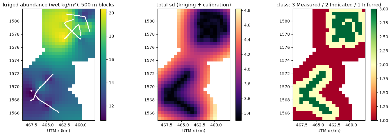
Everything below was produced by the pipeline from public GEOMAR SO268 data with no manual geology. It shows the SHAPE of the pilot deliverable; it is not a resource statement.
Per-image output for the whole corpus (34k rows, geolocated, with the GEOMAR reference values): so268_per_image_coverage_v3.csv
*Prepared by Ocean Map software 2026-09-21 for Competent Person review. NOT a signed resource statement. Structured to ISBA/21/LTC/15/Rev.1 Annex V (CRIRSCO-derived) Table-1 items; S-K 1300 §229.1302 mapping noted in brackets.*
Imagery from 12 OFOS profiles (40,476 images; GEOMAR SO268/1–2, 2019; CC-BY) and 36 box cores (0.25 m², Schoening & Gazis 2019) were used to estimate nodule abundance over the German-area survey corridors. Nodule coverage was read from every image by a convolutional model validated on held-out profiles; coverage and nodule size were calibrated to core abundance; abundance was kriged onto 500 m blocks; blocks were classified by data spacing.
| Class | Area (km²) | Mean abundance (wet kg/m²) | Block sd (kg/m²) | Tonnes (wet) | Tonnes (dry, 28 % moisture assumed) |
|---|---|---|---|---|---|
| Measured | 26.0 | 15.7 | ±3.4 | 408,654 | 294,231 |
| Indicated | 44.0 | 14.9 | ±3.7 | 655,685 | 472,093 |
| Inferred | 66.5 | 15.5 | ±4.2 | 1,027,751 | 739,981 |
USBL-positioned. Frames flagged by altitude/blur are excluded (quality flag in per-image table).
profiles: MAE 2.95 % coverage, R² 0.65. Known limitation: packed facies (>30 % coverage) MAE ≈ 8 %.
Abundance reported on a WET basis as measured on deck; dry tonnes use an assumed 28 % moisture (NORI convention) pending site moisture determination.
(sill/range/nugget [17.71, 12625.158, 3.012]) on 500 × 500 m blocks (UTM 11N). Block uncertainty = √(kriging variance + calibration variance).
Distance from block centre to nearest data node: ≤0.5 km Measured, ≤1.5 km Indicated, ≤3.5 km Inferred. These are illustrative spacings for a corridor survey; a grid survey would follow the NORI precedent (cores ≤7 km + photo infill ≤3.5 km → Measured).
Highest block uncertainty lies at corridor edges and in the 1574–1577 km northing gap between the two survey blocks (see sd map). Recommended: (i) 6–10 box cores at high-sd blocks with laser-scaled deck photographs to tighten the coverage→kg/m² calibration; (ii) AUV photo lines at 3.5 km spacing across the inter-corridor gap; (iii) backscatter acquisition to constrain buried nodules.
*To be completed and signed by the CP after review of the data, methods and this draft.*
block_model_v0.csv (per-block abundance, sd, class), block_model_v0.png, coverage_v3_all_images.csv (per-image), FINDINGS-calibration-v1.md.
Draft 2026-09-21 — Ocean Map. Data © GEOMAR/PANGAEA CC-BY.