Вибірка растрових даних із використанням точок або багатокутників

Попередження

This tutorial is now obsolete. A new and updated version is available at Sampling Raster Data using Points or Polygons (QGIS3)

Many scientific and environmental datasets come as gridded rasters. Elevation data (DEM) is also distributed as raster files. In these raster files, the parameter that is being represented is encoded as the pixel values of the raster. Often, one needs to extract the pixel values at certain locations or aggregate them over some area. This functionality is available in QGIS via two plugins - Point Sampling Tool and Zonal Statistics plugin.

Огляд завдання

Given a raster grid of maximum temperature in the US, we need to extract the temperature at all urban areas and also calculate the average temperature for each county in the US.

Додаткові навички

• Re-project a vector layer.

• Select and remove multiple layers from QGIS Table of Contents.

Отримання даних

NOAA’s Climate Prediction Center provides GIS data related to temperature and precipitation in the US. Download the latest grid filei for maximum temperatures. The file will be named us.tmax_nohads_ll_{YYYYMMDD}_float.tif

We will use a CSV file from 2013 US Gazetteer representing urban areas in the US. Download the Urban Areas Gazetteer File.

As we want to aggregate temperature over counties, we will use 2013 TIGER/Line Shapefiles. Download the Counties (and equivalents) shapefile.

Для зручності, ви можете безпосередньо завантажити копію наборів даних за допомогою посилання, що надане нижче:

us.tmax_nohads_ll_20140525_float.tif

2013_Gaz_ua_national.zip

tl_2013_us_county.zip

Data Sources: [NOAACPC], [USGAZETTEER] [TIGER]

Виконання

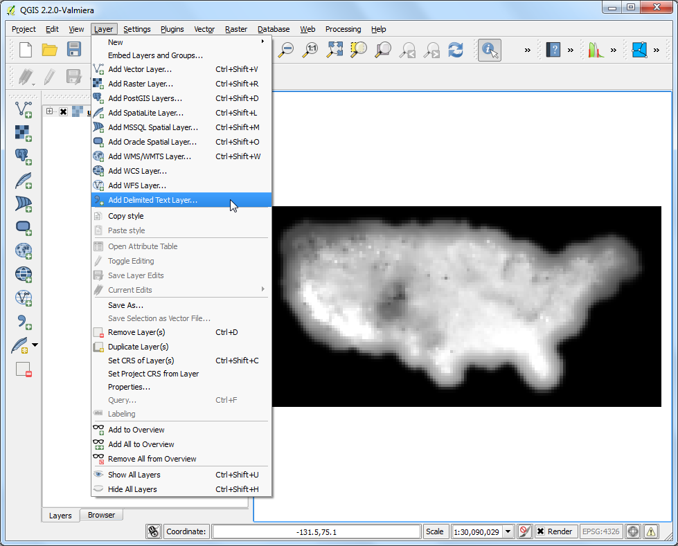
1. Go to Layer ‣ Add Raster Layer and browse to the downloaded us.tmax_nohads_ll_{YYYYMMDD}_float.tif file and click Open.

2. Once the layer is loaded, select the Identify tool and click anywhere on the layer. You will see the temperature value in celsius as the value or Band 1 at that location.

3. Now unzip the downloaded 2013_Gaz_ua_national.zip file and extract the 2013_Gaz_ua_national.txt file on your disk. Go to Layer ‣ Add Delimited Text Layer.

4. In the Create a Layer from Delimited Text File dialog, click Browse and open 2013_Gaz_ua_national.txt. Choose Tab under Custom delimiters. The point coordinates are in Latitude and Longitude, so select INTPTLONG as X field and INTPTLAT as Y field. Check the Use spatial index box and click OK.

5. Now we are ready to extract the temperature values from the raster layer. Install the Point Sampling Tool plugin. See Використання додатків for details on how to install plugins.

6. Open the plugin dialog from Plugins ‣ Analyses ‣ Point sampling tool.

7. In the Point Sampling Tool dialog, select 2013_Gaz_ua_national as the Layer containing sampling points. We must explicitely pick the fields from the input layer that we want in the output layer. Choose GEOID and NAME fields from the 2013_Gaz_ua_national layer. We can sample values from multiple raster band at once, but since our raster has only 1 band, choose the us.tmax_nohads_ll_{YYYYMMDD}_float: Band 1. Name the output vector layer as max_temparature_at_urban_locations.shp. Click the OK to start the sampling process. Click Close once the process finishes.

8. You will see a new layer max_temparature_at_urban_locations loaded in QGIS. Use the Identify tool to click on any point to see the attributes. You will see the us.tmax_no field - which contains the raster pixel value at the location of the point.

9. First part of our analysis is over. Let’s remove the unnecessary layers. Hold the Shift key and select max_temparature_at_urban_locations and 2013_Gaz_ua_national layers. Right-click and select Remove to remove them from QGIS TOC.

10. Go to Layer ‣ Add Vector Layer. Browse to the downloaded tl_2013_us_county.zip file and click Open. Select the tl_2013_us_county.shp as the layer and click OK.

11. The tl_2013_us_county will be added to QGIS. This layer is in EPSG:4269 NAD83 projection. This doesn’t match the projection of the raster layer. We will re-project this layer to EPSG:4326 WGS84 projection.

12. Right-click the tl_2013_us_county layer and select Save As...

13. In the Save Vector layer as.. dialog, click Browse and name the output file as counties.shp. Choose Selected CRS from the CRS dropdown menu. Click Browse and select WGS 84 as the CRS. Check the Add saved file to map and click OK.

14. A new layer named counties will be add to QGIS.

15. Enable the Zonal Statistics Plugins. This is a core plugin so it is already installed. See Використання додатків to know to how enable core plugins.

16. Go to Raster ‣ Zonal statistics ‣ Zonal statistics.

17. Select us.tmax_nohads_ll_{YYYYMMDD}_float as the Raster layer and counties as the Polygon layer containing the zones. Enter ZS_ as the Output column prefix. Click OK.

18. The analysis may take some time depending on the size of the dataset.

19. Once the processing finishes, select the counties layer. Use the Identify tool and click on any county polygon. You will see three new attributes added to the layer: ZS_count, ZS_mean and ZS_sum. These attributes contain the count of raster pixels, mean of raster pixel values and sum of raster pixel values respectively. Since we are interested in average temperature, the ZS_mean field will be the one to use.

20. Let’s style this layer to create a temperature map. Right-click the counties layer and select Properties.

21. Switch to the Style tab. Choose Graduated style and select ZS_mean as the Column. Choose a Color Ramp and Mode of your chose. Click Classify to create the classes. Click OK. (See Основи векторного моделювання for more details on styling.)

22. You will see the county polygons styled using average maximum temperature extracted from the raster grid.

---

If you want to report any issues with this tutorial, please comment below. (requires GitHub account)