Seasonal Water Yield

Summary

There is a high demand for tools estimating the effect of landscape management on the water supply service, for uses like irrigation, domestic consumption and hydropower production. While the InVEST Annual Water Yield model provides an estimate of total water yield for a catchment, many applications require knowledge of seasonal flows, especially during the dry season. This requires the understanding of hydrological processes in a catchment, in particular the partitioning between quickflow (occurring during or shortly after rain events) and baseflow (occurring during dry weather). In highly seasonal climates, baseflow is likely to provide greater value than quickflow, unless significant storage (e.g., a large reservoir) is available. The InVEST Seasonal Water Yield model seeks to provide guidance regarding the contribution of land parcels to the generation of both baseflow and quickflow. The model computes spatial indices that quantify the relative contribution of a parcel of land to the generation of both baseflow and quickflow. Currently, there are no quantitative estimates of baseflow, only the relative contributions of pixels; a separate tool is in development to address this question.

Introduction

Understanding the effect of landscape management on seasonal flow is of critical importance for watershed management. The contribution of a given parcel to streamflow depends on a number of environmental factors including climate, soil, vegetation, slope, and position along the flow path (determining if the pixel may receive water from upslope or if water recharged may later be evapotranspired).

Water flowing across the landscape is either evaporated, transpired, withdrawn by a well, or leaves the watershed as deep groundwater flow or streamflow. If we consider an individual pixel, and its value with respect to water yield, we can consider two approaches:

• The first gives credit to the net amount of water generated on a

  pixel as equal to the incoming precipitation minus the losses to evapotranspiration on that pixel. In this scheme, it is possible for actual evapotranspiration to be greater than precipitation if water is supplied to the site from upslope. Thus, the net generation could be negative. This approach pays no heed to the eventual disposition of that water generated on that pixel; that is, it does not consider whether the water actually shows up as streamflow or is evaporated or withdrawn somewhere along its path.

• The second approach gives credit to the water from a parcel that

  actually shows up as streamflow. Thus, if a parcel generates water that is later evaporated, the contribution is considered to be nil.

The former approach puts greater emphasis on the land-use and land-cover of a site, since the focus is on net generation from that pixel. It accounts for the subsidy of water from upslope pixels, but does not consider downslope effects. It represents the potential to generate streamflow (not an actual generation of flow).

The second approach puts more emphasis on the topographic position of a pixel, as that will determine the potential for water generated on that pixel to be consumed before becoming streamflow. It represents the actual streamflow generated by a pixel. Since actual streamflow cannot be less than zero, this approach, unlike the first, will result in indices that are greater than or equal to zero.

We use both of these concepts to develop a set of three indices, one for quickflow, one for recharge (which represents the ‘potential baseflow’), and one for actual baseflow. Here, baseflow is defined as the generation of streamflow with watershed residence times of months to years, while quickflow represents the generation of streamflow with watershed residence times of hours to days.

The Model

Quickflow

Quickflow (QF) is calculated using a method that combines the National Resources Conservation Service Curve Number (CN) method with an exponential distribution of monthly rainfall depths, as described in Guswa et al. 2018. Monthly rain events cause precipitation to fall on the landscape. Soil and land cover properties determine how much of the rain runs off of the land surface quickly (producing quickflow) versus infiltrating into the soil (producing local recharge.) The curve number is a simple way of capturing these soil + land cover properties - higher values of CN have higher runoff potential (for example, clay soils and low vegetation cover), lower values are more likely to infiltrate (for example, sandy soils and dense natural vegetation cover.)

To calculate quickflow, we use the mean event depth, \(\frac{P_{i,m}}{n_{i,m}}\) and assume an exponential distribution of daily precipitation depths on days with rain,

\[f\left( p \right) = \frac{1}{a_{i,m}}exp\left( - \frac{p}{a_{i,m}} \right)\]

Where \(a_{i,m} = \frac{P_{i,m}}{n_{m}}/25.4\) and

• \(a_{i,m}\) is the mean rain depth on a rainy day at pixel

  i on month m [in],

• \(n_{i,m}\) is the number of events at pixel i in month m

  [-],

• \(P_{i,m}\) is the monthly precipitation for pixel i at month

  m [mm].

Quickflow for pixels located in streams is set to the precipitation on that pixel, which assumes no infiltration, only runoff.

\[\text{QF}_{stream,m} = \ P_{stream,m}\]

otherwise it can be shown from the exponential distribution that the monthly runoff \(\text{QF}_{i,m}\) is

(88)\[\text{QF}_{i,m} = n_{m} \times \left( \left( a_{i,m} - S_{i} \right)\exp\left( - \frac{0.2S_{i}}{a_{i,m}} \right) + \frac{S_{i}^{2}}{a_{i,m}}\exp\left( \frac{0.8S_{i}}{a_{i,m}} \right)E_{1}\left( \frac{S_{i}}{a_{i,m}} \right) \right) \times \left( 25.4\ \left\lbrack \frac{\text{mm}}{\text{in}} \right\rbrack \right)\]

where

• \(S_{i}\) is the maximum potential retention, \(\frac{1000}{\text{CN}_{i}} - 10\) [in]

• \(\text{CN}_{i}\) is the curve number for pixel i

  [in^-1], tabulated as a function of the local LULC, and soil type (see Appendix I for a template of this table),

• \(E_{1}\) is the exponential integral function,

  \(E_{1}(x) = \int_{x}^{\infty}{\frac{e^{-t}}{t}\text{dt}}\).

• and \(25.4\) is a conversion factor from inches (used by the equation) to millimeters (used by the model)

(see Guswa et al. 2018).

A few edge cases are handled specially:

• When \(S_{i} = 0\), the \(E_{1}\) term goes to infinity. \(\text{QF}_{i,m}\) is set to zero in this case.

• To avoid issues with numerical instability when the result of exp becomes very large, when \(\frac{S_{i}}{a_{i,m}} > 100\), we round \(\text{QF}_{i,m}\) down to zero.

• With certain combinations of inputs, it is possible for the \(\text{QF}_{i,m}\) equation above to evaluate to a small negative number. In these cases \(\text{QF}_{i,m}\) is rounded to zero.

Thus the annual quick flow \(\text{QF}_{i}\), can be calculated from the sum of monthly \(\text{QF}_{i,m}\) values,

(89)\[\text{QF}_{i} = \sum_{m = 1}^{12}{QF_{i,m}}\]

Local recharge

The local recharge, or potential contribution to baseflow, of a pixel is computed from the local water balance. Precipitation that does not run off as quickflow, and is not evapotranspired by the vegetation on a pixel, can infiltrate the soil to become local recharge. Local recharge can be negative if a pixel does not receive enough of its own water to satisfy its vegetation requirements (determined by its crop factor Kc), so it uses water generated upslope of the pixel as well (referred to as an “upslope subsidy”.) The local recharge index is computed on an annual time scale, but uses values derived from monthly water budgets.

For a pixel i, the local recharge derived from the annual water budget is (Figure 1):

(90)\[L_{i} = P_{i} - \text{QF}_{i} - \text{AET}_{i}\]

Where annual actual evapotranspiration AET is the sum of monthly AET:

(91)\[\text{AET}_{i} = \sum_{\text{months}}^{}\text{AET}_{i,m}\]

For each month, \(\text{AET}_{i,m}\) is either limited by the demand (potential evapotranspiration - PET) or by the available water (from Allen et al. 1998):

(92)\[\text{AET}_{i,m} = min(\text{PET}_{i,m}\ ;\ P_{i,m} - \text{QF}_{i,m} + \alpha_{m}\beta_{i}L_{sum.avail,i})\]

Where \(\text{PET}_{i,m}\) is the monthly potential evapotranspiration,

(93)\[\text{PET}_{i,m} = K_{c,i,m} \times ET_{0,i,m}\]

\(L_{sum.avail,i}\) is recursively defined by (Figure 2),

(94)\[L_{sum.avail,i} = \sum_{j \in \{ neighbor\ pixels\ draining\ to\ pixel\ i\}}^{}{p_{\text{ij}} \cdot \left( L_{avail,j} + L_{sum.avail,j} \right)}\]

where \(p_{\text{ij}}\ \in \lbrack 0,1\rbrack\) is the proportion of flow from cell i to j, and \(L_{avail,i}\) is the available recharge to a pixel, which is \(L_{i}\) whenever \(L_{i}\) is negative, and a proportion \(\gamma\) of \(L_{i}\) when it is positive (see below for definition of \(\gamma\)):

(95)\[L_{avail,i}\ = min(\gamma L_{i},L_{i})\]

In the above:

• \(P_{i}\) and \(P_{i,m}\) are the annual and monthly

  precipitation, respectively [mm]

• \(\text{QF}_{i}\) and \(\text{QF}_{i,m}\) are the quickflow

  indices, defined above [mm]

• \(ET_{0,i,m}\) is the reference evapotranspiration for month m

  [mm]

• \(K_{c,i,m}\) is the monthly crop factor for the pixel’s LULC

• \(\alpha_{m}\) is the fraction of upslope annual available

  recharge that is available in month m (default is 1/12)

• \(\beta_{i}\) is the fraction of the upslope subsidy that is

  available for downslope evapotranspiration (default is 1; see Appendix II for more information)

• γ is the fraction of pixel recharge that is available to downslope

  pixels (default is 1)

Attribution of recharge

The total baseflow, \(Q_b\) (in mm), is the average of the contributing local recharges (negative or positive) in the catchment,

(96)\[Q_{b} = \frac{\sum_{k \in \left\{ \text{pixels in catchment} \right\}}^{}L_{k}}{n_{\text{pixels in catchment}}}\]

Attribution value to a pixel is the relative contribution of local recharge \(L\) on that pixel to the baseflow \(Q_b\):

(97)\[V_{R,i} = \frac{L_{i}}{{Q_{b} \times n}_{\text{pixels in catchment}}}\]

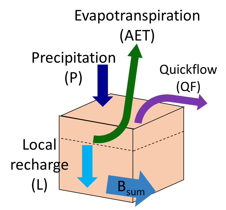
Figure 1. Water balance at the pixel scale to compute the local recharge (Eq. 3), where Bsum is the flow actually reaching the stream.

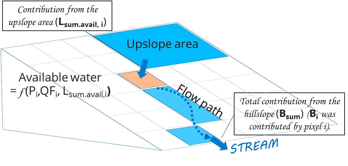
Figure 2. Routing at the hillslope scale to compute actual evapotranspiration (based on each pixel’s climate variables and the upslope contribution, see Eq. 5) and baseflow (based on Bsum, the flow actually reaching the stream, see Eq. 11-14)

Baseflow

The baseflow index represents the contribution of a pixel to baseflow (i.e. water that reaches the stream during the dry season). If the local recharge is negative, then the pixel did not contribute to baseflow so \(B\) is set to zero. If the pixel contributed to groundwater recharge, then \(B\) is a function of the amount of flow leaving the pixel and of the relative contribution to recharge of this pixel.

For a pixel that is not adjacent to the stream channel, the cumulative baseflow, \(B_{sum,i}\), is proportional to the cumulative baseflow leaving the adjacent downslope pixels minus the cumulative baseflow that was generated on that same downslope pixel (Figure 2):

(98)\[\begin{split}B_{sum,i} = L_{sum,i}\sum_{j \in \{\text{cells to which cell i pours}\}}^{}\begin{Bmatrix} p_{\text{ij}}\left( 1 - \frac{L_{avail,j}}{L_{sum,j}} \right)\frac{B_{sum,j}}{L_{sum,j} - L_{j}}\ \text{ if }j\text{ is a nonstream pixel} \\ p_{\text{ij}}\ \text{ if }j\text{ is a stream pixel} \\ \end{Bmatrix}\end{split}\]

At the watershed outlet (or at any pixel adjacent to the stream), the sum of baseflow generation \(B_{sum,i}\) over all upslope pixels is equal to the sum of local generation over the same pixels (because there is no further opportunity for the slow flow to be consumed before reaching the stream):

(99)\[B_{sum,outlet} = L_{sum,outlet}\]

where \(L_{sum,i}\) is the cumulative upstream recharge defined by

(100)\[L_{sum,i} = L_{i} + \sum_{j,\ all\ pixels\ draining\ to\ pixel\ i}^{}{L_{sum,j} \cdot p_{\text{ji}}}\]

and the baseflow, \(B_{i}\) can be directly derived from the proportion of the cumulative baseflow leaving cell i, with respect to the available recharge to the upstream cumulative recharge:

(101)\[B_{i} = max\left(B_{sum,i} \cdot \frac{L_{i}}{L_{sum,i}}, 0\right)\]

Calibration

It is always recommended to validate against observed data if possible. However, while the quickflow output from the model may be used as a quantitative measure, baseflow is intended to be used as an index, not an absolute value. So it is difficult to combine quickflow and baseflow and expect to get realistic model results for validating against observed flow. One possibility is to validate the relative values (i.e. the distribution of values across the landscape). This requires several (at least >3, more realistically >5) stream gauges, which can be compared with the quickflow and baseflow outputs of the model, aggregated to the same stream gauge points. Alternatively, results may be compared to a different spatially-explicit model, if it is available.

If you do try quantitatively validating either quickflow, or a combination of quickflow and baseflow (again, not recommended, but people do try), note that since the results are in millimeters, if we simply sum these up over the whole area, the result is likely to be orders of magnitude too large, and doesn’t represent the total water volume properly. Instead, use the mean B or Qf value across the watershed, convert millimeters to meters, then multiply by the watershed area to get a value in cubic meters, which can be compared against observed flow data. Alternatively, you could calculate volume per pixel and sum those.

See the paper Hamel et al (2020) for an example of calibrating the Seasonal Water Yield model against observed data and other hydrology models. For more general guidance about assessing uncertainty in ecosystem services analyses, see Hamel & Bryant (2017).

Limitations and Simplifications

Like all InVEST models, Seasonal Water Yield uses a simplified approach to estimating quickflow and baseflow, and does not include many of the complexities that occur as water moves through a landscape. Quickflow is primarily based on curve number, which does not take topography into account. For baseflow, although the model uses a physics-based approach, the equations are extremely simplified at both spatial and temporal scales, which significantly increases the uncertainty on the absolute numbers produced. So we do not suggest to use the absolute values, but instead the relative values across the landscapes (where we assume that the simplifications matter less, because they apply to the entire landscape).

Data Needs

Note

All spatial inputs must have exactly the same projected coordinate system (with linear units of meters), not a geographic coordinate system (with units of degrees).

Note

Raster inputs may have different cell sizes, and they will be resampled to match the cell size of the DEM. Therefore, all model results will have the same cell size as the DEM.

• Workspace (directory, required): The folder where all the model’s output files will be written. If this folder does not exist, it will be created. If data already exists in the folder, it will be overwritten.

• File Suffix (text, optional): Suffix that will be appended to all output file names. Useful to differentiate between model runs.

• Precipitation Directory (directory, conditionally required): Directory containing maps of monthly precipitation for each month. Only .tif files should be in this folder (no .tfw, .xml, etc files). Required if User-Defined Local Recharge is not selected.

  It is strongly recommended to use the same precipitation layers that were used to create the evapotranspiration input rasters. If they are based on different sources of precipitation data, this introduces another source of uncertainty in the data, and the mismatch could affect the water balance components computed by the model.

  Contents:

  • Precipitation (raster, units: mm/month, required): Twelve files, one for each month. File names must end with the month number (1-12). For example, the filenames ‘precip_1.tif’ and ‘precip1.tif’ are both valid names for the month of January.

• ET0 Directory (directory, conditionally required): Directory containing maps of reference evapotranspiration for each month. Only .tif files should be in this folder (no .tfw, .xml, etc files). Required if User-Defined Local Recharge is not selected.

  It is strongly recommended that the evapotranspiration input rasters be based on the same precipitation data as is input to the model. If they are based on different sources of precipitation data, this introduces another source of uncertainty in the data, and the mismatch could affect the water balance components computed by the model.

  Contents:

  • Reference Evapotranspiration (raster, units: mm/month, required): Twelve files, one for each month. File names must end with the month number (1-12). For example, the filenames ‘et0_1.tif’ ‘evapotranspiration1.tif’ are both valid for the month of January.

• Digital Elevation Model (raster, units: m, required): Map of elevation above sea level.

• Land Use/Land Cover (raster, required): Map of land use/land cover codes. Each land use/land cover type must be assigned a unique integer code. All values in this raster MUST have corresponding entries in the Biophysical Table.

• Soil Hydrologic Group (raster, conditionally required): Map of soil hydrologic groups. Pixels may have values 1, 2, 3, or 4, corresponding to soil hydrologic groups A, B, C, or D, respectively.

• Area of Interest (vector, polygon/multipolygon, required): A map of areas over which to aggregate and summarize the final results.

• Biophysical Table (CSV, required): A table mapping each LULC code to biophysical properties of the corresponding LULC class. All values in the LULC raster must have corresponding entries in this table.

  A .csv (Comma Separated Value) table containing model information corresponding to each of the land use classes in the LULC raster. All LULC classes in the LULC raster MUST have corresponding values in this table. Each row is a land use/land cover class and columns must be named and defined as follows:

  Columns:

  • lucode (integer, required): LULC codes from the LULC raster. Each code must be a unique integer.

  • cn_[SOIL_GROUP] (number, units: unitless, required): Curve number values for each combination of soil group and LULC class. Replace [SOIL_GROUP] with each soil group code A, B, C, D so that there is one column for each soil group. Curve number values must be greater than 0.

    Specifically, column names must be “CN_A”, “CN_B”, “CN_C” and “CN_D”.

  • kc_[MONTH] (number, units: unitless, required): Crop/vegetation coefficient (Kc) values for this LULC class in each month. Replace [MONTH] with the numbers 1 to 12 so that there is one column for each month.

    Specifically, column names must be “kc_1”, “kc_2” … “kc_12”.

Table 2 Example Biophysical Table

description	lucode	Kc_1	Kc_2	Kc_3	Kc_4	Kc_5	Kc_6	Kc_7	Kc_8	Kc_9	Kc_10	Kc_11	Kc_12	CN_A	CN_B	CN_C	CN_D
Urban and paved roads	1	0.4	0.4	0.4	0.4	0.4	0.4	0.4	0.4	0.4	0.4	0.4	0.4	76	85	89	91
Grass	3	1	1	1	1	1	1	1	1	1	1	1	1	49	69	79	84
General agriculture	5	0.75	0.75	0.4	0.3	0.7	0.7	1.15	1.15	0.5	0.4	0.3	0.3	67	78	85	89
Tea	6	0.95	0.95	0.95	0.95	0.95	0.95	0.95	0.95	0.95	0.95	0.95	0.95	43	65	76	82
Coffee	7	1.05	1.05	1.05	1.05	1.05	1.05	1.05	1.05	1.05	1.05	1.05	1.05	43	65	76	82
Forest	8	1	1	1	1	1	1	1	1	1	1	1	1	36	60	73	79
Water	9	1	1	1	1	1	1	1	1	1	1	1	1	99	99	99	99
Forest plantation	11	1	1	1	1	1	1	1	1	1	1	1	1	43	65	76	82
Unpaved road	18	0.4	0.4	0.4	0.4	0.4	0.4	0.4	0.4	0.4	0.4	0.4	0.4	77	86	91	94
Agroforestry	19	1	1	1	1	1	1	1	1	1	1	1	1	43	65	76	82

• Rain Events Table (CSV, conditionally required): A table containing the number of rain events for each month. Required if neither User-Defined Local Recharge nor User-Defined Climate Zones is selected.

  A rain event is defined as >0.1mm precipitation.

  Columns:

  • month (number, units: unitless, required): Values are the numbers 1-12 corresponding to each month, January (1) through December (12).

  • events (number, units: unitless, required): The number of rain events in that month.

  Example rain events table.

  month	events
  1	9
  2	9
  3	13
  4	21
  5	20
  6	10
  7	11
  8	12
  9	9
  10	14
  11	21
  12	13

• Threshold Flow Accumulation (number, units: number of pixels, required): The number of upslope pixels that must flow into a pixel before it is classified as a stream.

• Alpha_m Parameter (text, conditionally required): The proportion of upslope annual available local recharge that is available in each month. Required if Use Monthly Alpha Table is not selected.

  Default value: 1/12.

• Beta_i Parameter (ratio, required): The proportion of the upgradient subsidy that is available for downgradient evapotranspiration.

  Default value: 1.

• Gamma Parameter (ratio, required): The proportion of pixel local recharge that is available to downgradient pixels.

  Default value: 1.

• Flow Direction Algorithm (option, required): Flow direction algorithm to use.

  Options:

  • D8: D8 flow direction

  • MFD: Multiple flow direction

  Controls how water flow is modeled. With the D8 algorithm, all water on a given pixel flows to the neighboring pixel that is most steeply downslope. With the Multiple flow direction (MFD) algorithm, the water on a pixel flows to all of its downslope neighbors, weighted by how steeply downslope they are.

Advanced model options

The monthly Rain Events table is a simple way to provide rain events data. This assumes that there is one such number for the whole watershed, which may not be true for large areas or areas with very spatially variable precipitation.

To represent variability in the number of rain events, it is possible to enter a map of climate zones, and associated number of rain events for each zone.

Inputs

• Climate Zones (advanced) (true/false): Use user-defined climate zone data in lieu of a global rain events table.

• Climate Zone Table (CSV, conditionally required): Table of monthly precipitation events for each climate zone. Required if User-Defined Climate Zones is selected.

  Columns:

  • cz_id (integer, required): Climate zone ID numbers, corresponding to the values in the Climate Zones map.

  • [MONTH] (number, units: unitless, required): The number of rain events that occur in each month in this climate zone. Replace [MONTH] with the month abbreviations: jan, feb, mar, apr, may, jun, jul, aug, sep, oct, nov, dec, so that there is a column for each month.

  Example climate zone rain events table.

  cz_id	jan	feb	mar	apr	may	jun	jul	aug	sep	oct	nov	dec
  1	9	9	13	21	20	10	11	12	9	14	21	13
  2	9	9	12	19	18	10	10	11	9	12	19	11

• Climate Zone Map (raster, conditionally required): Map of climate zones. All values in this raster must have corresponding entries in the Climate Zone Table.

The model computes sequentially the local recharge layer, and then the baseflow layer from local recharge. Instead of InVEST calculating local recharge, this layer could be obtained from a different model (e.g, RHESSys.) To compute baseflow contribution based on your own recharge layer, it is possible to bypass the first part of the model and directly enter a map of local recharge.

Inputs

• User-defined Recharge Layer (advanced) (true/false): Use user-defined local recharge data instead of calculating local recharge from the other provided data.

• Local Recharge (raster, units: mm, conditionally required): Map of local recharge data. Required if User-Defined Local Recharge is selected.

The alpha parameter represents the temporal variability in the contribution of upslope available water to evapotranspiration on a pixel. In the default parameterization, its value is set to 1/12, assuming that the soil buffers water release and that the monthly contribution is exactly 1\12^th of the annual contribution.

To allow upslope subsidy to be temporally variable instead, the user can instead provide a table of monthly alpha values.

Inputs

• Use Monthly Alpha Table (advanced) (true/false): Use montly alpha values instead of a single value for the whole year.

• Monthly Alpha Table (CSV, conditionally required): Table of alpha values for each month. Required if Use Monthly Alpha Table is selected.

  Columns:

  • month (number, units: unitless, required): Values are the numbers 1-12 corresponding to each month.

  • alpha (number, units: unitless, required): The alpha value for that month.

Interpreting Results

The resolution of the output rasters will be the same as the resolution of the DEM that is provided as input.

• [Workspace] folder:

• Parameter log: Each time the model is run, a text (.txt) file will be created in the Workspace. The file will list the parameter values and output messages for that run and will be named according to the service, the date and time. When contacting NatCap about errors in a model run, please include the parameter log.

• B_[Suffix].tif (type: raster; units: mm, but should be interpreted as relative values, not absolute): Map of baseflow \(B\) values, the contribution of a pixel to slow release flow (which is not evapotranspired before it reaches the stream)

• B_sum_[Suffix].tif (type: raster; units: mm, but should be interpreted as relative values, not absolute): Map of \(B_{\text{sum}}\)values, the flow through a pixel, contributed by all upslope pixels, that is not evapotranspired before it reaches the stream

• CN_[Suffix].tif (type: raster): Map of curve number values

• L_avail_[Suffix].tif (type: raster; units: mm, but should be interpreted as relative values, not absolute): Map of available local recharge \(L_{\text{avail}}\)

• L_[Suffix].tif (type: raster; units: mm, but should be interpreted as relative values, not absolute): Map of local recharge \(L\) values

• L_sum_avail_[Suffix].tif (type: raster; units: mm, but should be interpreted as relative values, not absolute): Map of \(L_{\text{sum.avail}}\) values, the available water to a pixel, contributed by all upslope pixels, that is available for evapotranspiration by this pixel

• L_sum_[Suffix].tif (type: raster; units: mm, but should be interpreted as relative values, not absolute): Map of \(L_{\text{sum}}\) values, the flow through a pixel, contributed by all upslope pixels, that is available for evapotranspiration to downslope pixels

• QF_[Suffix].tif (type: raster; units: mm): Map of annual quickflow (QF) values

• P_[Suffix].tif (type: raster; units: mm/year): The total precipitation across all months on this pixel.

• Vri_[Suffix].tif (type: raster; units: mm): Map of the values of recharge (contribution, positive or negative), to the total recharge

• aggregated_results_swy_[Suffix].shp: Table containing biophysical values for each watershed, with fields as follows:

  • qb (units: mm, but should be interpreted as relative values, not absolute): Mean local recharge value within the watershed

  • vri_sum (units: mm): total recharge contribution, (positive or negative) within the watershed. The sum of Vri_[Suffix].tif pixel values within the watershed.

• [Workspace]\intermediate_outputs folder:

• aet_[Suffix].tif (type: raster; units: mm): Map of actual evapotranspiration (AET)

• qf_1_[Suffix].tif…qf_12_[Suffix].tif (type: raster; units: mm): Maps of monthly quickflow (1 = January… 12 = December)

• Si_[Suffix].tif (type: raster; units: inches): Maximum potential retention, used in the calculation of quickflow. (Note that the unit is converted to mm in Eq. (88)).

• stream_[Suffix].tif (type: raster): Stream network generated from the input DEM and Threshold Flow Accumulation. Values of 1 represent streams, values of 0 are non-stream pixels.

Appendix 1: Data sources and guidance for parameter selection

Precipitation

Evapotranspiration

Digital Elevation Model

Land Use/Land Cover

Soil Groups

Watersheds

Curve Number

Kc

Rain Events

Threshold Flow Accumulation

Flow Direction Algorithm

Climate Zones

Climate zone data is available on the Köppen-Geiger climate classification site.

You can also find InVEST-ready Climate Zone data on the NatCap Data Hub: https://data.naturalcapitalproject.stanford.edu/dataset/?_tags_limit=0&tags=CLIMATE+ZONES

alpha_m

Default: 1/12. See Appendix 2

beta_i

Default: 1. See Appendix 2

gamma

Default: 1. See Appendix 2

Appendix 2: Alpha, beta and gamma parameters - definition and alternative values

\(\alpha\) (alpha) and \(\beta_{i}\) (beta) represent the fraction of annual recharge from upslope pixels that is available to a downslope pixel for evapotranspiration in a given month. The product \(\alpha \times \beta_{i}\) is expected to be <1 since some water from upslope may be unavailable, either when it follows deep flowpaths or when the timing of supply and (evapotranspiration) demand is not synchronized.

\(\alpha\) is a function of precipitation seasonality: recharge from a given month can be used by downslope areas during later months, depending on the subsurface travel times. In the default parameterization, its value is set to 1/12, assuming that the soil buffers water release and that the monthly contribution is exactly one 12^th of the annual contribution. An alternative assumption is to set values to the antecedent monthly precipitation values, relative to the total precipitation: P_m-1/P_annual

\(\beta_{i}\) is a function of local topography and soils: for a given amount of upslope recharge, the amount of water used by a pixel is a function of the storage capacity. It also depends on the characteristics of the upslope area: the use of the upslope subsidy is conditioned by the shape and area of the contribution area (i.e. the recharge from the pixel just above the pixel of interest is less likely to be lost than the pixels much further away)

In the default parameterization, \(\beta\) is set to 1 for all pixels. One alternative is to set \(\beta_{i}\) as TI, the topographic wetness index for a pixel, defined as \(ln(\frac{A}{\text{tan}\beta}\)) (or other formulation including soil type and depth).

γ (gamma) represents the fraction of pixel recharge that is available to downslope pixels. It is a function of soil properties and possibly topography. In the default parameterization, γ is constant over the landscape and plays a role similar to \(\alpha\).

In practice

The options above are provided mainly for research purposes. In practice, we suggest that for highly seasonal climates, alpha should be set to the antecedent monthly precipitation values, relative to the total precipitation: P_m-1/P_annual

Then, we offer two options to address the uncertainty around the parameter values:

1. Verification of actual evapotranspiration with observations

The model outputs the actual evapotranspiration at the annual time scale: users can adjust parameters to meet observed actual evapotranspiration (e.g. from MODIS, https://www.ntsg.umt.edu/project/modis/mod16.php). In the following, “_mod” stands for modeled AET, “_obs” stands for observed AET.

• If AET_mod > AET_obs, the model overpredicts evapotranspiration,

  which can be corrected by: reducing Kc values, or reducing gamma values, and/or beta values (so less water is available for each pixel).

• If AET_mod < AET_obs, the model underpredicts evapotranspiration,

  which can be corrected by: increasing Kc values (and increasing gamma or beta values if they are not at their maximum of 1).

If monthly values of AET are available, a finer calibration can be performed by changing the seasonal parameter alpha.

2. Ensemble modeling

The model can be run under different assumptions and the outputs compared to estimate the effect of parameter error. Parameter ranges can be determined from assumptions about the proportion of upslope subsidy available to a given pixel; they can be set to the maximum bounds (0 and 1) for preliminary results.

References

Allen, R.G., Pereira, L.S., Raes, D., Smith, M., 1998. Crop evapotranspiration - Guidelines for computing crop water requirements, FAO Irrigation and drainage paper 56. Rome, Italy.

Guswa, A. J., Hamel, P., &amp; Meyer, K. (2018). Curve number approach to estimate monthly and annual direct runoff. Journal of Hydrologic Engineering, 23(2). https://doi.org/10.1061/(asce)he.1943-5584.0001606

Hamel, P. & Bryant, B. (2017). Uncertainty assessment in ecosystem services analyses: Seven challenges and practical responses. Ecosystem Services, Volume 24. https://doi.org/10.1016/j.ecoser.2016.12.008.

Hamel, P., Valencia, J., Schmitt, R., Shrestha, M., Piman, T., Sharp, R.P., Francesconi, W., Guswa, A.J., 2020. Modeling seasonal water yield for landscape management: Applications in Peru and Myanmar. Journal of Environmental Management 270, 110792.

NRCS-USDA, 2007. National Engineering Handbook. United States Department of Agriculture, https://www.nrcs.usda.gov/wps/portal/nrcs/detailfull/national/water/?cid=stelprdb1043063.