Urban Nature Access

Summary

Nature in urban areas provides important opportunities for recreation. The model for urban nature access provides a measure of both the supply of urban nature and the demand for nature by the urban population, ultimately calculating the balance between supply and demand. Both urban nature and population can optionally be divided into different groups. Supply is determined by the type, size, proximity, and quality of urban nature that is accessible per capita for recreational purposes. Demand is determined as natural space per capita, as typically required by policy or standards. The balance quantifies the extent to which supply meets demand, at the individual, administrative, and city level.

Introduction

Nature in urban areas provides important opportunities for recreation, along with social, psychological, and physical health benefits (Bratman et al. 2019, Keeler et al. 2019, Remme et al. 2021). As reviewed by Liu et al. (2022), assessing nature-based recreation requires an understanding of i) urban nature “supply”, which itself depends on availability and quality, and ii) urban nature “demand”, which depends on people’s preferences or policy requirements.

This InVEST model follows the structure described in Liu et al. (2022), by assessing the supply and demand for urban nature and the local supply-demand balance, which identifies areas with a surplus or deficit (positive or negative balance, respectively) of urban nature, with respect to a policy standard (Liu et al., 2022). In doing so, the model focuses on nature access in urban areas. Because the model is capable of modeling supply, demand, and balance of many types of urban nature, such as parks, greenspaces, wetlands, and shorelines, we refer to the model here as the urban nature access model. It is up to the user to choose which components of urban nature to include in their analysis.

The default model assesses overall urban nature supply, demand, and balance for the total urban population. In addition, three optional extensions of the core model can be used to provide more detailed results:

• Urban nature supply, demand, and balance can be summarized to

  different groups within the population (e.g., by different age groups, levels of income, race or ethnicity, etc.), which may be important for equity considerations. See Running the Model with Results Summarized by Population Groups

• For a more detailed understanding of the supply of urban nature, the

  user may optionally provide more detailed information on how far people are likely to travel to make use of different kinds of urban nature. For example, people may travel farther to visit large parks as compared to local pocket parks. See Running the Model with Radii Defined Per Urban Nature Class

• For a more detailed understanding of the supply of urban nature to

  different population groups, the user may optionally provide information on how far different groups are likely to travel to reach urban nature. For example, people who own cars may travel further to recreate than people who rely on public transit. See Running the Model with Radii Defined per Population Group

The Model

The model calculates urban nature access based on the location and amount of urban nature, the location and number of people, and the per-capita need or demand for urban nature. The area of urban nature in pixel \(j\) is represented as \(S_j\). Values of \(S_j\) are in square meters, where the proportion of the area of a pixel that is covered by urban nature is defined in the land use/land cover (LULC) Attribute Table. The population in pixel \(i\) is represented by \(P_i\). Per capita requirements for urban nature are specified as \(g_{cap}\), and are often based on policy targets. Together, these components are used to calculate the following three main metrics, described in greater detail in Running the Default Model:

• Urban nature supply: the amount of urban nature supplied to the

  population residing in a pixel

• Urban nature demand: the amount of urban nature required/demanded

  by the population in a pixel

• Urban nature balance: the difference between the urban nature supplied

  to a pixel and what is demanded by the population in that pixel

Decay Function

People use nature areas more frequently if they are closer to their homes (Andkjaer & Arvidsen, 2015). This frequency diminishes as distance increases. This is referred to as ‘distance decay’. The model describes this distance decay between urban nature and the population by the decay function \(f\left( d_{ij} \right)\) where \(d_{ij}\) is the distance between nature and a population pixel, and \(d_{0}\) is a user-defined search distance within which to search for nature pixels. Search distance is always Euclidean distance (straight-line distance between the center points of pixels A and B) and assumes square pixels.

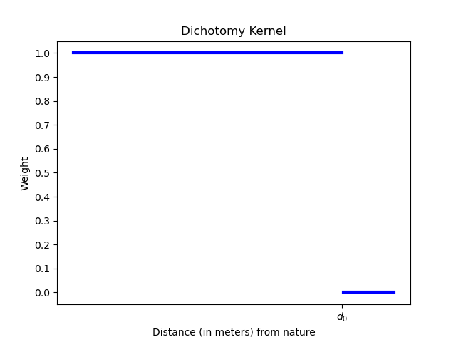
This model provides various distance-decay functions for the user to choose among, which are defined and illustrated in greater detail below. The dichotomy option treats all pixels within a set search distance from a pixel as equally accessible. This option is recommended when a policy for urban nature or greenspace targets a certain amount of nature within a particular distance from people’s residences. For example, the Netherlands set a target of at least \(60m^2\) urban nature per person within 500m of households (Roo et al. 2011).

For studies taking into account the decay of the service of urban nature, more realistically representing the probability to visit urban nature, the decay function should match available visitation data. Therefore, three additional distance-decay functions are available – exponential, Gaussian, and density. All assign more weight to urban nature located closer to people, reflecting people’s increased likelihood of visiting nature closer to them.

Dichotomy

The dichotomous kernel considers all pixels within the search distance \(d_{0}\) from a pixel with nature to be equally accessible.

\[\begin{split}\begin{align*} f(d_{ij}, d_0) &= \left\{\begin{array}{lr} 1 & \text{if} d_{ij} \leq d_0 \\ 0 & \text{if} d_{ij} > d_0 \\ \end{array}\right\} \\ \end{align*}\end{split}\]

Exponential

A distance-weighted exponential decay function, where people are more likely to visit the nature closest to them, with likelihood falling off exponentially out to the maximum radius \(d_{0}\).

\[\begin{split}\begin{align*} f(d_{ij}, d_0) &= \left\{\begin{array}{lr} e^{(-d_{ij}/d_0)} & \text{if} d_{ij} \leq d_0 \\ 0 & \text{if} d_{ij} \gt d_0 \\ \end{array}\right\} \\ \end{align*}\end{split}\]

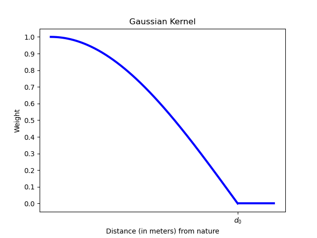
Gaussian

A distance-weighted decay function, where people are more likely to visit the nature closest to them, with likelihood decreasing according to a normal (“gaussian”) distribution with a sigma of 3, out to the maximum radius \(d_{0}\).

\[\begin{split}\begin{align*} f(d_{ij}, d_0) &= \left\{\begin{array}{lr} \frac{e^{-\frac{1}{2}\left ( \frac{d_{ij}}{d_0} \right )^2}-e^{-\frac{1}{2}}}{1-e^{-\frac{1}{2}}} & \text{if} d_{ij} \leq d_0 \\ 0 & \text{if} d_{ij} \gt d_0 \\ \end{array}\right\} \\ \end{align*}\end{split}\]

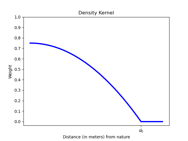
Density

A distance-weighted decay function, where people are more likely to visit the nature closest to them, with likelihood decreasing faster as distances appoach the search radius \(d_{0}\).

\[\begin{split}\begin{align*} f(d_{ij}, d_0) &= \left\{\begin{array}{lr} \frac{3}{4}\left(1-\left(\frac{d_{ij}}{d_{0}}\right)^{2}\right) & \text{if} d_{ij} \leq d_0 \\ 0 & \text{if} d_{ij} \gt d_0 \\ \end{array}\right\} \\ \end{align*}\end{split}\]

Running the Default Model

The default model assumes a uniform radius of travel (“search radius”) that is defined by the user, i.e. only nature within an X meter distance of someone’s home contributes to a person’s recreational benefit.

Calculating Urban Nature Supply

The calculation of urban nature supply to each population pixel uses the Two-Step Floating Catchment Area (2SFCA) method (Mao and Nekorchuk, 2013; Xing et al., 2018). Given an urban nature pixel \(j\), all population pixels with the search radius \(d_{0}\) are searched. The urban nature/population ratio \(R_{j}\) for this pixel is calculated using the nature pixel’s area \(S_{j}\) divided by the total population within the search radius, weighted according to the selected search kernel’s distance-based weighting. Then, centered on each pixel in the population raster, all the natural pixels within its distance-weighted catchment are searched. All of the \(R_{j}\) of these natural pixels are summed to calculate the urban nature supply per capita \(A_{i}\) to every population pixel. We take this approach for supply, rather than simply the amount of nature within a radius of a home, because using a gravity-based approach takes into account the weighted availability of nature. In other words, 2SFCA considers the context that a lot of people use greenspace which is common in a city area.

This can be graphically understood as:

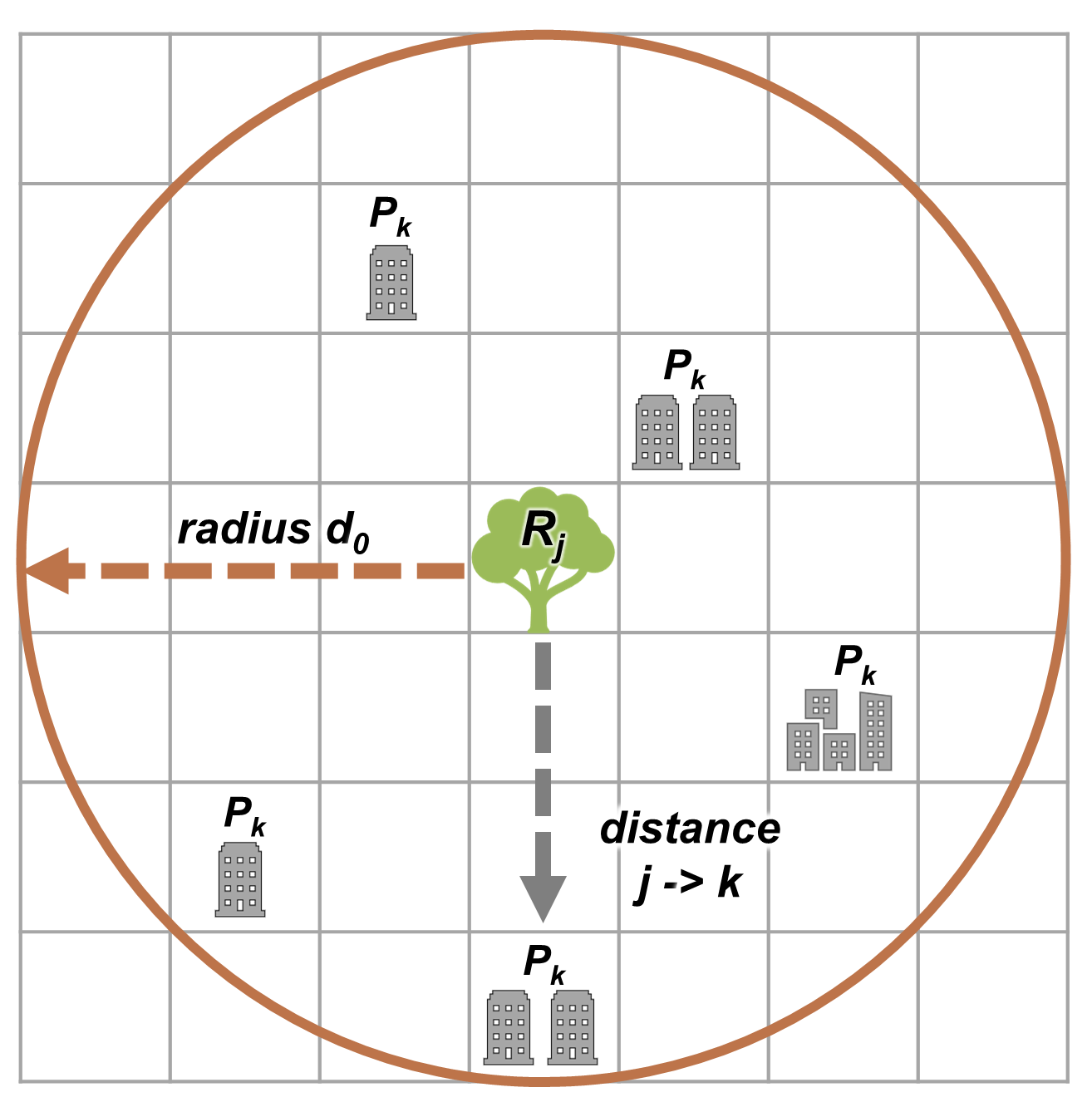
Fig. 14 Step 1: Locating populations within the search radius of urban nature.

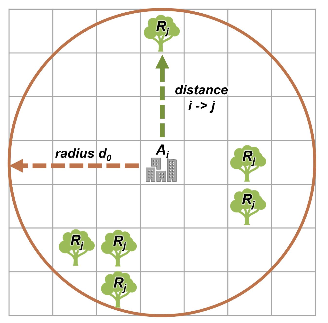
Fig. 15 Step 2: Locating urban nature within the search radius of populations.

More formally, the urban nature/population ratio \(R_{j}\) is defined as:

\[\begin{split}\begin{align*} R_j &= \left\{\begin{array}{lr} \frac{S_j}{\sum_{k \in \left\{d_{jk} \leq d_0 \right\}} P_k \cdot f(d_{jk})} & \text{if} P_k \cdot f(d_{jk}) >= 1 \\ S_j & \text{otherwise} \\ \end{array}\right\} \\ \end{align*}\end{split}\]

Where:

• \(R_{j}\) is the urban nature/population ratio of nature pixel \(j\).

• \(S_{j}\) is the area of nature in pixel \(j\)

• \(d_{0}\) is the search radius

• \(k\) is the population pixel within search radius of natural pixel \(j\)

• \(d_{jk}\) is the distance between natural pixel \(j\) and population pixel \(k\).

• \(P_{k}\) is the population of pixel \(k\).

• \(f(d)\) is the selected decay function.

Then, the urban nature/population ratio is weighted by the selected decay function and summed within the search radius to give greenspace supply, \(A_{i}\):

\[A_i = \sum_{j \in \left\{d_{ij} \leq d_0 \right\}} R_j \cdot f(d_{ij})\]

Where:

• \(i\) is any pixel in the population raster

• \(A_{i}\) is the urban nature per capita supplied to pixel \(i\) (square meters per person)

• \(d_{ij}\) is the distance between pixel \(i\) and natural pixel \(j\).

• \(d_{0}\) is the search radius

Calculate Urban Nature Demand

Derived from the population layer and the user-defined urban nature demand, this measures the amount of accessible urban nature required to adequately supply all people in each pixel.

\[demand_{i} = P_{i} \cdot g_{cap}\]

Where:

• \(i\) is a pixel

• \(demand_{i}\) is the required area of urban nature (in square meters) needed by the population residing at pixel \(i\) in order to fully satisfy their urban nature needs.

• \(P_{i}\) is the population (people per pixel) at pixel \(i\)

• \(g_{cap}\) is the user-defined per-capita urban nature requirement (square meters per person)

Calculate Urban Nature Balance

Local planning documents or urban planning goals often state that every resident in a region should be allocated a certain amount of nature, \(g_{cap}\). The per-capita urban nature supply/demand budget \(SUP\_ DEM_{i,cap}\) at pixel \(i\), is defined by assessing the balance between the supplied urban nature and the planning goal for nature (often greenspace) per capita per pixel:

\[SUP\_DEM_{i,cap} = A_i - g_{cap}\]

To determine the balance for all people in each pixel, \(SUP\_ DEM_{i,cap}\) is multiplied by the population \(P_{i}\) at pixel \(i\):

\[SUP\_DEM_{i} = SUP\_DEM_{i,cap} \cdot P_i\]

Calculate Accessible Urban Nature

It is often useful to find the total area within the given search radius, given by:

\[accessible_{i} = \sum_{j \in \left\{d_{ij} \leq d_{0} \right\}}{S_j \cdot f(d_{ij})}\]

Where \(accessible_{i}\) is the total area of urban nature accessible to pixel \(i\) within the search radius \(d_0\), weighted by the decay function.

Summarizing Outputs to Administrative Units

The user must provide a vector with administrative unit boundaries that may represent any district level that the user is interested in. These boundaries are needed to obtain administrative-level measurements.

The administrative level supply/demand balance is the sum of the balance of each pixel \(i\) within the administrative boundary \(adm\):

\[SUP\_DEM_{adm} = \sum_{i \in \left\{adm \right\}} SUP\_DEM_i\]

\(SUP\_ DEM_{adm}\) indicates how much urban nature, in square meters, is under- or over-supplied in an administrative unit.

The average per-capita urban nature supply/demand balance is also calculated at the administrative level:

\[SUP\_DEM_{adm,cap} = \frac{SUP\_DEM_{adm}}{P_{adm}}\]

Where \(P_{adm}\) is the total population within the administrative boundary.

When \(SUP\_ DEM_{i,cap} < 0\) on any given pixel \(i\), it indicates that people in this pixel are under-supplied with urban nature. Summing up these populations across all pixels within an administrative unit provides the number of people in an administrative unit with an urban nature deficit, \(Pund_{adm}\), relative to the recommended urban nature \(g_{cap}\):

\[\begin{split}Pund_{adm} = \sum_{i \in \{adm\}} \left\{ \begin{array}{lr} P_{i} & \text{if} SUP\_DEM_{i,cap} < 0 \\ 0 & \text{otherwise} \\ \end{array} \right\}\end{split}\]

Similarly, the same rationale is applied to find the number of people with an urban nature surplus in an administrative unit, \(Povr_{adm}\), relative to the recommended urban nature \(g_{cap}\):

\[\begin{split}Povr_{adm} = \sum_{i \in \{adm\}} \left\{ \begin{array}{lr} P_{i} & \text{if} SUP\_DEM_{i,cap} > 0 \\ 0 & \text{otherwise} \\ \end{array} \right\}\end{split}\]

Running the Model with Radii Defined Per Urban Nature Class

Urban nature has different types. Pocket parks provide convenient recreation experience nearby, while municipal parks attract people from more distant places. If the user has data to split the types of urban nature and to adjust the travel distance for each type of urban nature, the accessibility of each type of urban nature to pixel \(i\) can be calculated using the class-specific radius. These urban nature types and their associated search radii are provided to the model by user input in the Land Use Land Cover (LULC) attribute table. Each type of LULC classification marked as urban nature will be calculated separately in order to give more detailed results concerning the accessible urban nature of each type. It is up to the user to decide how to split the urban nature.

If \(r\) is the type of urban nature, \(j\) is an urban nature pixel of \(r\) type, \(d_{0,r}\) is the search radius for \(r\) type of urban nature , then the urban nature/population ratio for this urban nature type is calculated by the area of this urban nature divided by the population within the radius weighted by the user’s selection of distance-weighted decay function:

\[R_{j,r} = \frac{S_{j,r}}{ \sum_{k \in \{d_{kj} \leq d_{0,r}\}}{P_k \cdot f(d_{jk})} }\]

The accessibility of urban nature type \(r\), \(A_{i,r}\) to pixel \(i\) is calculated by summing up the distance-weighted \(R_{j,r}\) within the search radius:

\[A_{i,r} = \sum_{j \in d_{ij} \leq d_{0,r}}{R_{j,r} \cdot f(d_{ij})}\]

The total urban nature supplied to pixel \(i\), \(A_{i}\) is calculated by adding up the \(A_{i,r}\) across all types of urban nature:

\[A_i = \sum_{r=1}^{r}{A_{i,r}}\]

Accessible urban nature in this mode is calculated by:

\[accessible_{i,r} = \sum_{j \in \left\{d_{ij} \leq d_{0,r} \right\}}{S_{j,r} \cdot f(d_{ij})}\]

Where \(accessible_{i,r}\) is the total area of urban nature of class \(r\) accessible within the search radius, weighted by the decay function. \(S_{j,r}\) is the area of urban nature on pixel \(j\) of urban nature class \(r\).

Other steps and outputs are the same as in the core model.

Running the Model with Results Summarized by Population Groups

The user has the option to provide population characteristics indicating the proportion of the total population that belong to a given population group within each administrative unit. Examples of population groups might be age or income brackets. The user will decide how to split the population according to data availability and the study objective.

To analyze the supply-demand balance for certain groups within the general population, an additional calculation is done for each group \(gn\), given the proportion of the group in the total population of an administrative unit, \(Rp,gn\).

For the undersupplied population within group \(gn\) and administrative unit \(adm\), this is defined as:

\[Pund_{adm,gn} = Pund_{adm} \cdot Rp,gn\]

And for the oversupplied population within group \(gn\) and administrative unit \(adm\):

\[Povr_{adm,gn} = Povr_{adm} \cdot Rp,gn\]

The user may wish to conduct further correlation analysis between population characteristics and the above outputs to see if certain groups of people are associated with deficit or surplus urban nature supply at different levels.

Running the Model with Radii Defined per Population Group

The search radius has an important impact on urban nature supply and different populations have different radii. For example, people with a car can travel further for recreation, or elderly people may travel shorter distances (Liu et al., 2022). This group-specific search radius \(d_{0,gn}\), is defined by the user for each group \(gn\) along with the proportion of the total population within an administrative unit belonging to this group. Given these two group-specific pieces of information, the urban nature supplied to each group in a pixel, \(A_{i,gn}\) can be obtained.

First, the urban nature area will be divided among the population within its search radius, \(R_{j}\). Since different groups have different radii (see Figure below), the total served population is the sum of each group within their respective search radius. Population at pixel \(i\) consists of different groups. The size of the group \(gn\) in pixel \(i\) is calculated by:

\[P_{i,gn} = P_i \cdot Rp,gn\]

where \(P_{i}\) is the population at pixel \(i\), and \(Rp,gn\) is the proportion of this group in the total population within each individual administrative unit.

\[R_j = \frac{S_j}{ \sum_{gn=1}^{gn} \left( \sum_{k \in \{d_{kj} \leq d_{0,gn} \}}{ P_{k,gn} \cdot f(d_{jk})} \right) }\]

Fig. 16 Urban nature provides service to older adults within d0, g1 (the radius for this population group), and provides service to younger adults within d0, g2 (the radius for that population group).

Urban nature supply to group \(gn\) by pixel \(i\) is calculated by (and conceptually exemplified in the Figure below):

\[A_{i,gn} = \sum_{j \in \{d_{ij} \leq d_{0,gn}\}} R_j \cdot f(d_{ij})\]

Fig. 17 Aged population only receive service from greenspace within d0, g1, i.e., greenspace A; Younger adults receive service from greenspaces within d0, g2, i.e., greenspace A and greenspace B.

The average urban nature supply per capita to pixel \(i\) is calculated by a weighted sum of \(A_{i,gn}\):

\[A_i = \sum_{n=1}^{n}{A_{i,gn} \cdot Rp,gn}\]

The per-capita urban nature balance at pixel \(i\), \(SUP\_ DEM_{i,cap}\) is defined by assessing the difference between the supplied urban nature to pixel \(i\) and the user-defined planning goal for urban nature per capita, \(g_{cap}\):

\[SUP\_DEM_{i,cap} = A_i - g_{cap}\]

The per-capita urban nature balance of group \(gn\) at pixel \(i\) (\(SUP\_ DEM_{i,cap,gn}\)) is defined by assessing the difference between the supplied urban nature to group \(gn\) at pixel \(i\) and the planning goal for urban nature per capita, \(g_{cap}\):

\[SUP\_DEM_{i,cap,gn} = A_{i,gn} - g_{cap}\]

\(P_{i,gn}\) is the population of group \(gn\) at pixel \(i\). The population of the group \(gn\) in pixel \(i\) multiplied by the per capita urban nature balance of the same group, (\(SUP\_ DEM_{i,cap,gn}\)), will give the urban nature area supply-demand balance of that group at pixel \(i\). Summing the supply-demand balance of all groups at pixel i will generate the supply-demand balance for all people at pixel i (\(SUP\_ DEM_{i}\)).

\[SUP\_DEM_i = \sum_{gn=1}^{gn}{SUP\_DEM_{i,cap,gn} \cdot P_{i,gn}}\]

Summing the supply-demand balance at each pixel within administrative units will result in the administrative level supply-demand balance.

\[SUP\_DEM_{adm} = \sum_{i=1}^{i}{SUP\_DEM_i}\]

To give an administrative level per capita urban nature supply-demand balance, administrative level urban nature supply and demand balance \(SUP\_ DEM_{adm}\) is divided by the total population of the administrative unit \(P_{adm}\):

\[SUP\_DEM_{adm,cap} = \frac{SUP\_DEM_{adm}}{P_{adm}}\]

To calculate the average per-capita supply-demand balance of group \(gn\) with an administrative unit \(adm\), the model multiplies the greenspace balance \(SUP\_ DEM_{i,cap,gn}\) by the population of group \(gn\) at pixel \(i\), and then summed up for all pixels in \(adm\) and divided by the population of group \(gn\) within \(adm\).

\[SUP\_DEM_{adm,cap,gn} = \frac{ \sum_{i \in \{adm\}}{SUP\_DEM_{i,cap,gn} \cdot P_{i,gn}} }{ P_{adm,gn} }\]

To analyze the supply-demand balance for certain groups within the general population, an additional calculation is done.

The population of group \(gn\) who has a urban nature deficit within administrative unit \(adm\) is given by:

\[\begin{split}Pund_{adm,gn} = \sum_{i \in \{adm\}} \left\{ \begin{array}{lr} P_{i,gn} & \text{if} SUP\_DEM_{i,cap,gn} < 0 \\ 0 & \text{otherwise} \\ \end{array} \right\}\end{split}\]

The total under-supplied population within administrative unit \(adm\) is given by:

\[Pund_{adm} = \sum_{gn=1}^{gn}{Pund_{adm,gn}}\]

The population of group \(gn\) who has a urban nature surplus within administrative unit \(adm\) is given by:

\[\begin{split}Povr_{adm,gn} = \sum_{i \in \{adm\}} \left\{ \begin{array}{lr} P_{i,gn} & \text{if} SUP\_DEM_{i,cap,gn} > 0 \\ 0 & \text{otherwise} \\ \end{array} \right\}\end{split}\]

The total over-supplied population within administrative unit \(adm\) is given by:

\[Povr_{adm} = \sum_{gn=1}^{gn}{Povr_{adm,gn}}\]

Accessible urban nature in this mode is calculated by:

\[accessible_{i,gn} = \sum_{j \in \left\{d_{ij} \leq d_0 \right\}} S_{j,gn} \cdot f(d_{ij})\]

Where \(accessible_{i,gn}\) is the total area of urban nature accessible to population group \(gn\) within the search radius, weighted by the decay function. \(S_{j,gn}\) is the area of urban nature on pixel \(j\) accessible to group \(gn\).

Limitations and Simplifications

Search distances (radii) are Euclidian (straight-line), the model does not consider roads or other real-world walking/transportation constraints.

The model does not take into account the total size of greenspace patches, it only evaluates the different greenspace classes and their attributes per pixel. A workaround for this is to define different land use classes based on size, such as “small parks” and “large parks”. Then you can define a different visitation radius for each size class.

Demand uses a generic calculation (m2 per capita), while citites often take different approaches to quantifying demand. Additionally, there are no official international metrics for demand that can be easily applied, so local knowledge is needed.

Model output can be used as a proxy for recreation and health benefits, but it is not an ideal indicator for the complexity of human-nature relationships.

Data Needs

Note

Sample data are supplied to provide examples of requirements and formatting.

Note

All spatial inputs must be in the same projected coordinate system and in linear meter units. Outputs will be resampled to match the squared-off resolution and spatial projection of the LULC.

• Workspace (directory, required): The folder where all the model’s output files will be written. If this folder does not exist, it will be created. If data already exists in the folder, it will be overwritten.

• File Suffix (text, optional): Suffix that will be appended to all output file names. Useful to differentiate between model runs.

• Land Use/Land Cover (raster, required): A map of LULC codes. All values in this raster must have corresponding entries in the LULC attribute table. For this model in particular, the urban nature types are of importance. Non-nature types are not required to be uniquely identified. All outputs will be produced at the resolution of this raster.

• LULC Attribute Table (CSV, required): A table identifying which LULC codes represent urban nature. All LULC classes in the Land Use Land Cover raster MUST have corresponding values in this table. Each row is a land use land cover class.

  Columns:

  • lucode (integer, required): LULC codes from the LULC raster. Each code must be a unique integer.

  • urban_nature (ratio, required): The proportion (0-1) indicating the naturalness of the land types. 0 indicates the naturalness level of this LULC type is lowest (0% nature), while 1 indicates that of this LULC type is the highest (100% nature)

  • search_radius_m (number, units: m, conditionally required): The distance within which a LULC type is relevant to the population group of interest. This is the search distance that the model will apply for this LULC type. Values must be >= 0 and defined in meters. Required when running the model with search radii defined per urban nature class.

• Population Raster (raster, units: count, required): A raster representing the number of inhabitants per pixel.

• Administrative Boundaries (vector, polygon/multipolygon, required): A vector representing administrative units. Polygons representing administrative units should not overlap. Overlapping administrative geometries may cause unexpected results and for this reason should not overlap.

  Fields:

  • pop_[POP_GROUP] (ratio, conditionally required): The proportion of the population within each administrative unit belonging to the identified population group (POP_GROUP). At least one column with the prefix ‘pop_’ is required when aggregating output by population groups.

  Example attribute table for an administrative boundaries vector with 3 geometries:

  pop_male	pop_female
  0.56	0.44
  0.42	0.58
  0.38	0.62

• Urban Nature Demand Per Capita (number, units: m², required): The amount of urban nature that each resident should have access to. This is often defined by local urban planning documents.

• Decay Function (option, required): Pixels within the search radius of an urban nature pixel have a distance-weighted contribution to an urban nature pixel according to the selected distance-weighting function.

  Options:

  • Density: Contributions to an urban nature pixel decrease faster as distances approach the search radius. Weights are calculated by “weight = 0.75 * (1-(pixel_dist / search_radius)^2)”

  • Dichotomy: All pixels within the search radius contribute equally to an urban nature pixel.

  • Exponential: Contributions to an urban nature pixel decrease exponentially, where “weight = e^(-pixel_dist / search_radius)”

  • Gaussian: Contributions to an urban nature pixel decrease according to a normal (“gaussian”) distribution with a sigma of 3.

• Search Radius Mode (option, required): The type of search radius to use.

  Options:

  • Radius defined per population group: The search radius is defined for each distinct population group.

  • Radius defined per urban nature class: The search radius is defined for each distinct urban nature LULC classification.

  • Uniform radius: The search radius is the same for all types of urban nature.

• Aggregate By Population Groups (true/false): Whether to aggregate statistics by population group within each administrative unit. If selected, population groups will be read from the fields of the user-defined administrative boundaries vector. This option is implied if the search radii are defined by population groups.

• Uniform Search Radius (number, units: m, conditionally required): The search radius to use when running the model under a uniform search radius. Required when running the model with a uniform search radius. Units are in meters.

• Population Group Radii Table (CSV, conditionally required): A table associating population groups with the distance in meters that members of the population group will, on average, travel to find urban nature. Required when running the model with search radii defined per population group.

  Columns:

  • pop_group (text, optional): The name of the population group. Names must match the names defined in the administrative boundaries vector.

  • search_radius_m (number, units: m, conditionally required): The search radius in meters to use for this population group. Values must be >= 0.

  Example of a table matching the groups in the administrative boundaries vector above:

  pop_group	search_radius_m
  pop_male	900
  pop_female	1200

Interpreting Results

Output Folder

• output/urban_nature_supply_percapita.tif The calculated supply of urban

  nature. Units: urban nature per capita supplied to pixel i (square meters per person).

• outputs/urban_nature_demand.tif The required area of urban nature

  needed by the population residing each pixel in order to fully satisfy their urban nature needs. Higher values indicate a greater demand for accessible urban nature from the surrounding area. Units: square meters urban nature per pixel.

• output/urban_nature_balance_percapita.tif The pixel-level value

  of urban nature balance per capita. Positive pixel values indicate an oversupply of urban nature relative to the stated urban nature demand. Negative values indicate an undersupply of urban nature relative to the stated urban naturedemand. This output is of particular interest to interpret where individuals are most nature deprived. Units: Square meters of urban nature deficit or oversupply per person.

• outputs/urban_nature_balance_totalpop.tif The urban nature balance

  for the total population in a pixel. Positive pixel values indicate an oversupply of urban nature relative to the stated urban nature demand. Negative values indicate an undersupply of urban nature relative to the stated urban nature demand. This output is of particular relevance to understand the total amount of nature deficit for the population in a particular pixel. Units: square meters of urban nature deficit or oversupply per pixel.

• output/admin_boundaries.gpkg A copy of the user’s administrative

  boundaries vector with a single layer.

  • SUP_DEMadm_cap - the average urban nature supply/demand balance

    available per person within this administrative unit.

  • Pund_adm - the total population within the administrative unit

    that is undersupplied with urban nature.

  • Povr_adm - the total population within the administrative unit

    that is oversupplied with urban nature.

  If the user has selected to aggregate results by population group

  and has elected to run the model with search radii define either as a uniform distance or per urban nature class, these additional fields will be created:

  • Pund_adm_[POP_GROUP] - the total population belonging to the

    population group POP_GROUP within this administrative unit that are undersupplied with urban nature.

  • Povr_adm_[POP_GROUP] - the total population belonging to the

    population group POP_GROUP within this administrative unit that is oversupplied with urban nature.

  If the user has elected to run the model with search radii defined per

  population group, these additional fields will be created.

  • Pund_adm_[POP_GROUP] - see description above.

  • Povr_adm_[POP_GROUP] - see description above.

  • SUP_DEMadm_cap_[POP_GROUP] - the average urban nature supply/demand

    balance available per person in population group POP_GROUP within this administrative unit.

  Note that the field SUP_DEMadm_cap_[POP_GROUP] is only created if the user elected to run the model with search radii defined per population group.

Other files in the output directory vary depending on the selected search radius mode:

Uniform Search Radius

• output/accessible_urban_nature.tif - the area of urban nature accessible

  within the provided search radius, weighted by the decay function. Units: square meters.

Search Radii Defined per Urban Nature Class

• output/accessible_urban_nature_lucode_[LUCODE].tif - the area of urban

  nature of class LUCODE within the provided search radius for this lucode, weighted by the decay function. Units: square meters.

Search Radii Defined per Population Group

• output/accessible_urban_nature_to_[POP_GROUP].tif - the area of urban

  nature accessible to the population group POP_GROUP given the search radius for the population group, weighted by the decay function. Units: square meters.

Intermediate Folder

These files will be produced in every search radius mode:

• intermediate/aligned_lulc.tif A copy of the user’s land use land

  cover raster. If the user-supplied LULC has non-square pixels, they will be resampled to square pixels.

• intermediate/aligned_population.tif The user’s population raster,

  aligned to the same resolution and dimensions as the aligned LULC. Units: people per pixel.

• intermediate/undersupplied_population.tif Each pixel represents

  the population in the total population that are experiencing an urban nature deficit. Units: people per pixel.

• intermediate/oversupplied_population.tif Each pixel represents

  the population in the total population that are experiencing an urban nature surplus. Units: people per pixel.

Other files found in the intermediate directory vary depending on the selected search radius mode:

Uniform Search Radius

• intermediate/distance_weighted_population_within_[SEARCH_RADIUS].tif

  A sum of the population within the given search radius SEARCH_RADIUS, weighted by the user’s decay function. Units: people per pixel.

• intermediate/urban_nature_area.tif Pixels values represent the

  area of urban nature(in square meters) represented in each pixel. Units: square meters.

• intermediate/urban_nature_population_ratio.tif The calculated

  urban nature/population ratio.

Search Radii Defined per Urban Nature Class

• intermediate/distance_weighted_population_within_[SEARCH_RADIUS].tif

  A sum of the population within the given search radius SEARCH_RADIUS, weighted by the user’s decay function. Units: people per pixel.

• intermediate/urban_nature_area_[LUCODE].tif Pixel values

  represent the area of urban nature(in square meters) represented in each pixel for the urban nature class represented by the land use land cover code LUCODE. Units: square meters.

• intermediate/urban_nature_population_ratio_lucode_[LUCODE].tif

  The calculated urban nature/population ratio calculated for the urban nature class represented by the land use land cover code LUCODE. Units: square meters per person

• intermediate/urban_nature_supply_percapita_lucode_[LUCODE].tif The urban

  nature supplied to populations due to the land use land cover class LUCODE. Units: square meters per person

Search Radii Defined per Population Group

• output/urban_nature_balance_[POP_GROUP].tif Positive pixel values

  indicate an oversupply of urban nature relative to the stated urban nature demand to the population group POP_GROUP. Negative values indicate an undersupply of urban nature relative to the stated urban nature demand to the population group POP_GROUP. Units: Square meters of urban nature per person.

• intermediate/urban_nature_area.tif Pixels values represent the

  area of greenspace (in square meters) represented in each pixel. Units: square meters.

• intermediate/population_in_[POP_GROUP].tif Each pixel represents

  the population of a pixel belonging to the population in the population group POP_GROUP. Units: people per pixel.

• intermediate/proportion_of_population_in_[POP_GROUP].tif Each

  pixel represents the proportion of the total population that belongs to the population group POP_GROUP. Units: proportion between 0 and 1.

• intermediate/distance_weighted_population_in_[POP_GROUP].tif Each pixel

  represents the total number of people within the search radius for this population group POP_GROUP, weighted by the user’s selection of decay function. Units: people per pixel.

• intermediate/distance_weighted_population_all_groups.tif The total

  population, weighted by the appropriate decay function. Units: people per pixel.

• intermediate/urban_nature_supply_percapita_to_[POP_GROUP].tif The urban

  nature supply to the population group POP_GROUP. Units: square meters per person.

• intermediate/undersupplied_population_[POP_GROUP].tif Each pixel

  represents the population in population group POP_GROUP that are experiencing an urban nature deficit. Units: people per pixel.

• intermediate/oversupplied_population_[POP_GROUP].tif Each pixel

  represents the population in population group POP_GROUP that are experiencing an urban nature surplus. Units: people per pixel.

Appendix: Data Sources

Land Use/Land Cover

Population raster

Multiple regional and global datasets exist that estimate population size and density at high resolution, such as:

• WorldPop global population data: https://www.worldpop.org/methods/populations/

• Meta/CIESIN global population density data: https://dataforgood.facebook.com/dfg/tools/high-resolution-population-density-maps

• European 100-m population data: https://www.eea.europa.eu/data-and-maps/data/population-density-disaggregated-with-corine-land-cover-2000-2

Urban greenspace data

Multiple regional and global datasets exist that (help) define urban nature, including the following:

• Latin American cities: https://www.nature.com/articles/s41597-022-01701-y

• European cities: https://land.copernicus.eu/local/urban-atlas

• Global data:

  • http://data.ess.tsinghua.edu.cn/

  • https://www.openstreetmap.org/

(For comparison, see: https://www.sciencedirect.com/science/article/abs/pii/S1618866722001819)

Urban nature demand

There is no set global standard for urban nature demand. A commonly suggested value is 9m2, that is often credited incorrectly to the WHO (see https://www.researchgate.net/post/I-see-many-studies-citing-WHO-for-their-international-minimum-standard-for-green-space-9m2-per-capita-But-where-is-the-actual-study/4 for discussion on this value). Papers providing overviews of demand values and discussion around these values include Liu et al. (2022), Liu et al. (2021), and Badiu et al. (2016).

References

Andkjaer S., Arvidsen J. 2015. Places for active outdoor recreation - a scoping review. Journal of Outdoor Recreation and Tourism, 12, 25-46. https://doi.org/10.1016/j.jort.2015.10.001

Badiu, D.L., Ioja, C.I., Patroescu, M., Breuste, J., Artmann, M., Nita, M.R., Gradinaru, S.R., Hossu, C.A., Onose, D.A. 2016. Is urban green space per capita a valuable target to achieve cities’ sustainability goals? Romania as a case study. Ecological Indicators 70, 53-66. https://doi.org/10.1016/j.ecolind.2016.05.044

Bratman, G. N., Anderson, C. B., Berman, M. G., Cochran, B., De Vries, S., Flanders, J., … & Daily, G. C. 2019. Nature and mental health: An ecosystem service perspective. Science advances, 5(7), eaax0903. https://doi.org/10.1126/sciadv.aax0903

Keeler, B. L., Hamel, P., McPhearson, T., Hamann, M. H., Donahue, M. L., Meza Prado, K. A., … & Wood, S. A. 2019. Social-ecological and technological factors moderate the value of urban nature. Nature Sustainability, 2(1), 29-38. https://doi.org/10.1038/s41893-018-0202-1

Liu, H., Remme, R.P., Hamel, P., Nong, H., Ren, H., 2020. Supply and demand assessment of urban recreation service and its implication for greenspace planning-A case study on Guangzhou. Landsc. Urban Plan. 203, 103898. https://doi.org/10.1016/j.landurbplan.2020.103898

Liu H., Hamel P., Tardieu L., Remme R.P., Han B., Ren H., 2022. A geospatial model of nature-based recreation for urban planning: Case study of Paris, France. Land Use Policy, https://doi.org/10.1016/j.landusepol.2022.106107.

Mao L. and Nekorchuk D., 2013. Measuring spatial accessibility to health care for populations with multiple transportation modes. Health & Place 24, 115–122. https://doi.org/10.1016/j.healthplace.2013.08.008

Remme, R. P., Frumkin, H., Guerry, A. D., King, A. C., Mandle, L., Sarabu, C., … & Daily, G. C. 2021. An ecosystem service perspective on urban nature, physical activity, and health. Proceedings of the National Academy of Sciences, 118(22), e2018472118. https://doi.org/10.1073/pnas.2018472118

Roo, M. D., Kuypers, V. H. M., & Lenzholzer, S. 2011. The green city guidelines: techniques for a healthy liveable city. The Green City. http://library.wur.nl/WebQuery/wurpubs/fulltext/178666

Xing L.J, Liu Y.F, Liu X.J., 2018. Measuring spatial disparity in accessibility with a multi-mode method based on park green spaces classification in Wuhan, China. Applied Geography 94, 251–261. https://doi.org/10.1016/j.apgeog.2018.03.014