Carbon Storage and Sequestration

Summary

Terrestrial ecosystems, which store more carbon than the atmosphere, are vital to influencing carbon dioxide-driven climate change. The InVEST Carbon Storage and Sequestration model uses maps of land use along with stocks in four carbon pools (aboveground biomass, belowground biomass, soil and dead organic matter) to estimate the amount of carbon currently stored in a landscape or the amount of carbon sequestered over time. Additional data on the market or social value of sequestered carbon and its annual rate of change, and a discount rate can be used to optionally estimate the value of this ecosystem service to society. Limitations of the model include an oversimplified carbon cycle, an assumed linear change in carbon sequestration over time, and potentially inaccurate discounting rates.

Introduction

Ecosystems regulate Earth’s climate by adding and removing greenhouse gases (GHG) such as CO₂ from the atmosphere. Forests, grasslands, peat swamps, and other terrestrial ecosystems collectively store much more carbon than does the atmosphere (Lal 2002). By storing this carbon in wood, other biomass, and soil, ecosystems keep CO₂ out of the atmosphere, where it would contribute to climate change. Beyond just storing carbon, many systems also continue to accumulate it in plants and soil over time, thereby “sequestering” additional carbon each year. Disturbing these systems with fire, disease, or vegetation conversion (e.g., land use / land cover (LULC) conversion) can release large amounts of CO₂. Other management changes, like forest restoration or alternative agricultural practices, can lead to the storage of large amounts of CO₂. Therefore, the ways in which we manage terrestrial ecosystems are critical to regulating our climate.

Terrestrial-based carbon sequestration and storage is perhaps the most widely recognized of all ecosystem services (Stern 2007, IPCC 2006, Canadell and Raupach 2008, Capoor and Ambrosi 2008, Hamilton et al. 2008, Pagiola 2008). The social value of a sequestered ton of carbon is equal to the social damage avoided by not releasing the ton of carbon into the atmosphere (Tol 2005, Stern 2007). Calculations of social cost are complicated and controversial (see Weitzman 2007 and Nordhaus 2007b), but have resulted in value estimates that range from USD $9.55 to $84.55 per metric ton of CO₂ released into the atmosphere (Nordhaus 2007a and Stern 2007, respectively).

Managing landscapes for carbon storage and sequestration requires information about how much and where carbon is stored, how much carbon is sequestered or lost over time, and how shifts in land use affect the amount of carbon stored and sequestered over time. Since land managers must choose among sites for protection, harvest, or development, maps of carbon storage and sequestration are ideal for supporting decisions influencing these ecosystem services.

Such maps can support a range of decisions by governments, NGOs, and businesses. For example, governments can use them to identify opportunities to earn credits for reduced (carbon) emissions from deforestation and degradation (REDD). Knowing which parts of a landscape store the most carbon would help governments efficiently target incentives to landowners in exchange for forest conservation. Additionally, a conservation NGO may wish to invest in areas where high levels of biodiversity and carbon sequestration overlap (Nelson et al. 2008). A timber company may also want to maximize its returns from both timber production and REDD carbon credits (Plantinga and Birdsey 1994).

The Model

Carbon storage on a land parcel largely depends on the sizes of four carbon pools: aboveground biomass, belowground biomass, soil, and dead organic matter. The InVEST Carbon Storage and Sequestration model aggregates the amount of carbon stored in these pools according to land use maps and classifications provided by the user. Aboveground biomass comprises all living plant material above the soil (e.g., bark, trunks, branches, leaves). Belowground biomass encompasses the living root systems of aboveground biomass. Soil organic matter is the organic component of soil, and represents the largest terrestrial carbon pool. Dead organic matter includes litter as well as lying and standing dead wood.

Using maps of land use and land cover types and the amount of carbon stored in carbon pools, this model estimates the net amount of carbon stored in a land parcel over time and the market value of the carbon sequestered in remaining stock. Limitations of the model include an oversimplified carbon cycle, an assumed linear change in carbon sequestration over time, and potentially inaccurate discounting rates. Biophysical conditions important for carbon sequestration such as photosynthesis rates and the presence of active soil organisms are also not included in the model.

How it Works

The model maps carbon storage densities to land use/land cover (LULC) rasters which may include types such as forest, pasture, or agricultural land. The model summarizes results into raster outputs of storage, sequestration and value, as well as aggregate totals.

For each LULC type, the model requires an estimate of the amount of carbon in at least one of the four fundamental pools described above. If you have data for more than one pool, the modeled results will be more complete. The model simply applies these estimates to the LULC map to produce a map of carbon storage in the carbon pools included.

If you provide both a current and future LULC map, then the net change in carbon storage over time (sequestration and loss) and its social value can be calculated. To estimate this change in carbon sequestration over time, the model is simply applied to the current landscape and a projected future landscape, and the difference in storage is calculated, pixel by pixel. If multiple future scenarios are available, the differences between the current and each alternate future landscape can be compared.

Additionally if you provide a REDD scenario landcover map, the model will treat that raster as an additional future scenario, calculate storage and sequestration and summarize results.

Outputs of the model are expressed as Mg of carbon per pixel, and if desired, the value of sequestration in currency units per pixel. We strongly recommend using the social value of carbon sequestration if you are interested in expressing sequestration in monetary units. The social value of a sequestered ton of carbon is the social damage avoided by not releasing the ton of carbon into the atmosphere.

The valuation model estimates the economic value of sequestration (not storage) as a function of the amount of carbon sequestered, the monetary value of each unit of carbon, a monetary discount rate, and the change in the value of carbon sequestration over time. Thus, valuation can only be done in the carbon model if you have a future scenario. Valuation is applied to sequestration, not storage, because market prices relate only to carbon sequestration. Discount rates are multipliers that typically reduce the value of carbon sequestration over time. The first type of discounting, the standard economic procedure of financial discounting, reflects the fact that people typically value immediate benefits more than future benefits due to impatience and uncertain economic growth. The second discount rate adjusts the social value of carbon sequestration over time. This value will change as the impact of carbon emissions on expected climate change-related damages changes. If we expect carbon sequestered today to have a greater impact on climate change mitigation than carbon sequestered in the future this second discount rate should be positive. On the other hand, if we expect carbon sequestered today to have less of an impact on climate change mitigation than carbon sequestered in the future this second discount rate should be negative.

REDD Scenario Analysis

The carbon model can optionally perform scenario analysis according to a framework of Reducing Emissions from Forest Degradation and Deforestation (REDD) or REDD+. REDD is a scheme for emissions reductions under which countries that reduce emissions from deforestation can be financially compensated. REDD+ builds on the original REDD framework by also incorporating conservation, sustainable forest management, and enhancement of existing carbon stocks.

To perform REDD scenario analysis, the model requires three LULC maps: one for the current scenario, one for a future baseline scenario, and one for a future scenario under a REDD policy. The future baseline scenario is used to compute a reference level of emissions against which the REDD scenario can be compared. Depending on the specifics on the desired REDD framework, the baseline scenario can be generated in a number of different ways; for instance, it can be based on historical rates of deforestation or on projections. The REDD policy scenario map reflects future LULC under a REDD policy to prevent deforestation and enhance carbon sequestration.

Based on these three LULC maps for current, baseline, and REDD policy scenarios, the carbon biophysical model produces rasters for total carbon storage for each of the three LULC maps, and two sequestration rasters for future and REDD scenarios.

Limitations and Simplifications

The model simplifies the carbon cycle which allows it to run with relatively little information, but also leads to important limitations. For example, the model assumes that none of the LULC types in the landscape are gaining or losing carbon over time. Instead it is assumed that all LULC types are at some fixed storage level equal to the average of measured storage levels within that LULC type. Under this assumption, the only changes in carbon storage over time are due to changes from one LULC type to another. Therefore, any pixel that does not change its LULC type will have a sequestration value of 0 over time. In reality, many areas are recovering from past land use or are undergoing natural succession. The problem can be addressed by dividing LULC types into age classes (essentially adding more LULC types), such as three ages of forest. Then, parcels can move from one age class to the other in scenarios and change their carbon storage values as a result.

A second limitation is that because the model relies on carbon storage estimates for each LULC type, the results are only as detailed and reliable as the LULC classification used and carbon pool values supplied. Carbon storage clearly differs among LULC types (e.g., tropical forest vs. open woodland), but often there can also be significant variation within an LULC type. For example, carbon storage within a “tropical moist forest” is affected by temperature, elevation, rainfall, and the number of years since a major disturbance (e.g., clear-cut or forest fire). The variety of carbon storage values within coarsely defined LULC types can be partly recovered by using an LULC classification system and related carbon pool table which stratifies coarsely defined LULC types with relevant environmental and management variables. For example, forest LULC types can be stratified by elevation, climate bands or time intervals since a major disturbance. Of course, this more detailed approach requires data describing the amount of carbon stored in each of the carbon pools for each of the finer LULC classes.

Another limitation of the model is that it does not capture carbon that moves from one pool to another. For example, if trees in a forest die due to disease, much of the carbon stored in aboveground biomass becomes carbon stored in other (dead) organic material. Also, when trees are harvested from a forest, branches, stems, bark, etc. are left as slash on the ground. The model assumes that the carbon in wood slash “instantly” enters the atmosphere.

Finally, while most sequestration follows a nonlinear path such that carbon is sequestered at a higher rate in the first few years and a lower rate in subsequent years, the model’s economic valuation of carbon sequestration assumes a linear change in carbon storage over time. The assumption of a constant rate of change will tend to undervalue the carbon sequestered, as a nonlinear path of carbon sequestration is more socially valuable due to discounting than a linear path (Figure 1).

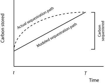
Figure 1: The model assumes a linear change in carbon storage (the solid line), while the actual path to the year :math:`T`’s carbon storage level may be non-linear (like the dotted line). In this case :math:`t` can indicate the year of the current landscape and :math:`T` the year of the future landscape. With positive discounting, the value of the modeled path (the solid line) is less valuable than the actual path. Therefore, if sequestration paths tend to follow the dotted line, the modeled valuation of carbon sequestration will underestimate the actual value of the carbon sequestered.

Data Needs

This section outlines the specific data used by the model. See the Appendix for additional information on data sources and pre-processing. Please consult the InVEST sample data (located in the folder where InVEST is installed, if you also chose to install sample data) for examples of all of these data inputs. This will help with file type, folder structure and table formatting. Note that all GIS inputs must be in the same projected coordinate system and in linear meter units.

• Current land use/land cover (required): Raster of land use/land cover (LULC) for each pixel, where each unique integer represents a different land use/land cover class. All values in this raster MUST have corresponding entries in the Carbon Pools table.

• Current Landcover Calendar Year (required for sequestration and valuation): The year depicted by the Current LULC map, for use in calculating sequestration and economic values.

• Carbon pools (required): A CSV (comma-separated value) table of LULC classes, containing data on carbon stored in each of the four fundamental pools for each LULC class. If information on some carbon pools is not available, pools can be estimated from other pools, or omitted by leaving all values for the pool equal to 0. The table must contain the following columns:

  • lucode: Unique integer for each LULC class (e.g., 1 for forest, 3 for grassland, etc.) Every value in the LULC map MUST have a corresponding **lucode* value in the Carbon Pool table.*

  • c_above: Carbon density in aboveground biomass [units: megagrams/hectare]

  • c_below: Carbon density in belowground biomass [units: megagrams/hectare]

  • c_soil: Carbon density in soil [units: megagrams/hectare]

  • c_dead: Carbon density in dead matter [units: megagrams/hectare]

Example: Hypothetical study with five LULC classes. Class 1 (Forest) contains the most carbon in all pools. In this example, carbon stored in above- and below-ground biomass differs strongly among land use classes, but carbon stored in soil varies less dramatically.

lucode	LULC_name	C_above	C_below	C_soil	C_dead
1	Forest	140	70	35	12
2	Coffee	65	40	25	6
3	Pasture/grass	15	35	30	4
4	Shrub/undergrowth	30	30	30	13
5	Open/urban	5	5	15	2

• Future landcover (required for sequestration and valuation): Raster of land use/land cover (LULC) for each pixel, where each unique integer represents a different land use/land cover class. All values in this raster MUST have corresponding entries in the Carbon Pools table.

• Future Landcover Calendar Year (required for sequestration and valuation): The year depicted by the Future LULC map, for use in calculating sequestration and economic values.

• REDD Policy (required for REDD sequestration and valuation): Raster of land use/land cover (LULC) for each pixel, where each unique integer represents a different land use/land cover class. All values in this raster MUST have corresponding entries in the Carbon Pools table.

• Economic data (required for valuation):

  • Price/Metric ton of carbon (\(V\) in the equation below): Price given in currency per metric ton of elemental carbon (not CO:sub:`2`). For applications interested in estimating the total value of carbon sequestration, we recommend value estimates based on damage costs associated with the release of an additional ton of carbon - the social cost of carbon (SCC). Stern (2007), Tol (2009), and Nordhaus (2007a) present estimates of SCC. For example, two SCC estimates we have used from Tol (2009) are $66 and $130 (in 2010 US dollars) (Polasky et al. 2010).

  • Market discount in Price of Carbon (\(r\) in the equation below): An integer percentage value which reflects society’s preference for immediate benefits over future benefits. One default value is 7% per year, which is one of the market discount rates recommended by the U.S. government for cost-benefit evaluation of environmental projects. However, this rate will depend on the country and landscape being evaluated, and should be selected based on local requirements. Philosophical arguments have been made for using a lower discount rate when modeling climate change related dynamics, which users may consider using. If the rate is set equal to 0% then monetary values are not discounted.

  • Annual rate of change in the price of carbon (\(c\) in the equation below): An integer percentage value which adjusts the value of sequestered carbon as the impact of emissions on expected climate change-related damages changes over time. Setting this rate greater than 0% suggests that the societal value of carbon sequestered in the future is less than the value of carbon sequestered now. It has been widely argued that GHG emissions need to be curtailed immediately to avoid crossing a GHG atmospheric concentration threshold that would lead to a 3 degree Celsius or greater change in global average temperature by 2105. Some argue that such a temperature change would lead to major disruptions in economies across the world (Stern et al. 2006). Therefore, any mitigation in GHG emissions that occurs many years from now may have no effect on whether or not this crucial concentration threshold is passed. If this is the case, C sequestration in the far future would be relatively worthless and a carbon discount rate greater than zero is warranted. Alternatively, setting the annual rate of change less than 0% (e.g., -2%) suggests that the societal value of carbon sequestered in the future is greater than the value of carbon sequestered now (this is a separate issue than the value of money in the future, a dynamic accounted for with the market discount rate). This may be the case if the damages associated with climate change in the future accelerate as the concentration of GHGs in the atmosphere increases.

The value of carbon sequestration over time for a given parcel x is:

(1)\[value\_seq_x=V\frac{sequest_x}{yr\_fut-yr\_cur}\sum^{yr\_fut-yr\_cur-1}_{t=0}\frac{1}{\left(1+\frac{r}{100}\right)^t\left(1+\frac{c}{100}\right)^t}\]

Running the Model

To launch the Carbon model navigate to the Windows Start Menu -> All Programs -> InVEST [version] -> Carbon. The interface does not require a GIS desktop, although the results will need to be explored with any GIS tool such as ArcGIS or QGIS.

This model supports avoided re-computation. This means the model will detect intermediate and final results from a previous run in the specified workspace and it will avoid re-calculating any outputs that are identical to the previous run. This can save significant processing time for successive runs when only some input parameters have changed.

Interpreting Results

The following is a short description of each of the outputs from the Carbon model. These results are found within the model’s Workspace specified in the user interface. In the file names below, “Suffix” refers to the optional user-defined Suffix input to the model.

• [Workspace] folder:

  • Parameter log: Each time the model is run, a text (.txt) file will be created in the Workspace. The file will list the parameter values and output messages for that run and will be named according to the service, the date and time. When contacting NatCap about errors in a model run, please include the parameter log.

  • report_[Suffix].html: This file presents a summary of all data computed by the model. It also includes descriptions of all other output files produced by the model, so it is a good place to begin exploring and understanding model results. Because this is an HTML file, it can be opened with any web browser.

  • tot_c_cur_[Suffix].tif/tot_c_fut_[Suffix].tif/tot_c_redd_[Suffix].tif: Rasters showing the amount of carbon stored in Mg in each pixel for the current, future and REDD scenarios. It is a sum of all of the carbon pools provided by the biophysical table.

  • delta_cur_fut_[Suffix].tif/delta_cur_redd_[Suffix].tif: Rasters showing the difference in carbon stored between the future/REDD landscape and the current landscape. The values are in Mg per pixel. In this map some values may be negative and some positive. Positive values indicate sequestered carbon, negative values indicate carbon that was lost.

  • npv_fut_[Suffix].tif/npv_redd_[Suffix].tif:** Rasters showing the economic value of carbon sequestered between the current and the future/REDD landscape dates. The units are in currency per pixel.

• [Workspace]\intermediate_outputs folder:

  • c_above_[Suffix].tif: Raster of aboveground carbon values, mapped from the Carbon Pools table to the LULC.

  • c_below_[Suffix].tif: Raster of belowground carbon values, mapped from the Carbon Pools table to the LULC.

  • c_dead_[Suffix].tif: Raster of dead carbon values, mapped from the Carbon Pools table to the LULC.

  • c_soil_[Suffix].tif: Raster of soil carbon values, mapped from the Carbon Pools table to the LULC.

  • _tmp_work_tokens: This directory stores metadata used iternally to enable avoided re-computation. No model results are stored here.

Appendix: Data Sources

This is a rough compilation of data sources and suggestions for finding, compiling, and formatting data. This section should be used for ideas and suggestions only. This section is updated as new data sources and methods become available.

Land use/land cover

Global land use data is available from:

• NASA: https://lpdaac.usgs.gov/dataset_discovery/modis/modis_products_table/mcd12q1 (MODIS multi-year global landcover data provided in several classifications)

• The European Space Agency: https://www.esa-landcover-cci.org (Three global maps for the 2000, 2005 and 2010 epochs)

• The University of Maryland?s Global Land Cover Facility: http://glcf.umd.edu/data/landcover/ (data available in 1 degree, 8km and 1km resolutions).

Data for the U.S. is provided by the USGS and Department of the Interior via the National Land Cover Database: https://www.mrlc.gov/finddata.php

The simplest categorization of LULCs on the landscape involves delineation by land cover only (e.g., cropland, temperate conifer forest, prairie). Several global and regional land cover classifications are available (e.g., Anderson et al. 1976), and often detailed land cover classification has been done for the landscape of interest.

A slightly more sophisticated LULC classification could involve breaking relevant LULC types into broad age categories (e.g., forest of age 0-10 years, 11-20, 21-40, etc.). This would allow separate estimates of carbon storage for different ages. In scenarios, parcels can move from one age class to the next, crudely capturing changes in carbon storage over time. This approach requires more information, however, including carbon storage estimates for each age class for all modeled pools of carbon.

A still more detailed classification could stratify LULC types by variables known to affect carbon storage within a given LULC type (e.g., montane forest 800-1000m, montane forest 1001-1200m, etc.). Rainfall, temperature, and elevation all typically influence carbon storage and sequestration (e.g., Jenny 1980, Coomes et al. 2002, Raich et al. 2006). If data are available to estimate carbon storage at different elevations, or at different levels of rainfall, temperature or other climate variables, model results will be substantially more accurate. This will typically take a large sample of plot estimates of carbon storage.

Carbon pools

Carbon storage data should be set equal to the average carbon storage values for each LULC class. The ideal data source for all carbon stocks is a set of local field estimates, where carbon storage for all relevant stocks has been directly measured. These can be summarized to the LULC map, including any stratification by age or other variable. If these data are not available, however, there are several general data sources that can be used.

Note that several sources, including IPCC (2006), report in units of biomass, while InVEST uses mass of elemental carbon. To convert metric tons of biomass to metric tons of C, multiply by a conversion factor, which varies typically from 0.43 to 0.51. Conversion factors for different major tree types and climatic regions are listed in Table 4.3 on page 4.48 of IPCC (2006).

Carbon stored in aboveground biomass

A good but very general source of data for carbon storage is the Intergovernmental Panel on Climate Change’s (IPCC) 2006 methodology for determining greenhouse gas inventories in the Agriculture, Forestry and Other Land Use (AFOLU) sector (http://www.ipcc-nggip.iges.or.jp/public/2006gl/pdf/4_Volume4/V4_02_Ch2_Generic.pdf, IPCC 2006). To use this set of information from the IPCC, you must know your site’s climate domain and region; use data from Table 4.1 on page 4.46 and a digital copy of the Food and Agriculture Organization of the United Nations’ (FAO) eco-region map (http://www.fao.org/geonetwork/srv/en/main.home) to figure that out. Tables 5.1 through 5.3 (p. 5.9) of IPCC (2006) give estimates for aboveground biomass in agriculture land with perennial woody biomass (e.g., fruit orchards, agroforestry, etc.). Tables 4.7, 4.8, and 4.12 give aboveground biomass estimates for natural and plantation forest types. Ruesch and Gibbs (2008) mapped the IPCC (2006) aboveground biomass carbon storage data given year 2000 land cover data, which can be accessed here: https://cdiac.ess-dive.lbl.gov/epubs/ndp/global_carbon/carbon_documentation.html.

Other general sources of carbon storage estimates can be found. For example, Grace et al. (2006) estimate the average aboveground carbon storage (leaf + wood) for major savanna ecosystems around the world (Table 1). Houghton (2005) gives aboveground carbon storage for natural and plantation forest types, by continent (Tables 1 and 3). Brown et al. (1989) give aboveground biomass estimates for tropical broadleaf forests as a function of land-use: undisturbed, logged and nonproductive (Table 7). Region-specific sources of carbon storage data are also available. Those we’ve found include:

• Latin America: Malhi et al. (2006) report aboveground biomass volumes for 227 lowland forest plots in Bolivia, Brazil, Colombia, Ecuador, French Guinea, Guyana, Panama, Peru, and Venezuela. Nascimento and Laurance (2002) estimate aboveground carbon stocks in twenty 1-ha plots of Amazonian rainforest. Tiessen et al. (1998) find aboveground carbon stocks for the Brazilian savanna types Caatingas and Cerrados.

• Africa: Zhang and Justice (2001) report aboveground carbon stocks for major forest and shrub LULC types for central African countries. Tiessen et al. (1998) estimates total aboveground biomass of degraded savanna in Senegal. Makundi (2001) reports mean annual incremental growth for three forest plantation types in Tanzania. Malimbwi et al. (1994) estimates aboveground carbon stocks in the miombo woodlands of Kitungalo Forest Reserve Tanzania. Munishi and Shear (2004) report aboveground carbon stocks in the Afromontane rain forests of the Eastern Arc Mountains of Tanzania. Glenday (2006) estimates aboveground carbon stocks for 3 forest types in the Kakamega National Forest of western Kenya.

• North America: Smith et al. (2006) estimate aboveground carbon stocks for all major forest types in the US.

• The Carbon On Line Estimator (http://www.ncasi2.org/COLE/) is a tool for calculating carbon characteristics in U.S. forests based on USDA Forest Service Forest Inventory & Analysis and Resource Planning Assessment data. With this tool, carbon characteristics can be examined at the scale of counties. Using the variables tab, aboveground, belowground, soil, or dead wood carbon pools can be selected.

• Coomes et al. (2002) estimate aboveground carbon stocks for native shrubland and forest types in New Zealand.

Aboveground biomass (and therefore carbon stocks) can also be calculated from timber inventories, which are often done by forestry ministries on a set of plots. Use the following formula to estimate the aboveground carbon stock in a forest stand that has been inventoried for its merchantable volume where VOB is the per-hectare volume of trees in cubic meters measured from tree stump to crown point (the merchantable portion of the tree), WD is the wood density of trees (dry biomass per unit of tree volume), BEF is the ratio of total aboveground dry biomass to dry biomass of inventoried volume, and CF is the ratio of elemental carbon to dry biomass, by mass (Brown 1997). The biomass expansion factor (BEF) accounts for C stored in all other portions of the tree aboveground (e.g., branches, bark, stems, foliage, etc; the non-merchantable portions of the tree). In most cases WD for a plot is approximated with values for dominant species. Brown (1997) provides a table of WD values for many tree species in Appendix 1 of section 3 and a method for calculating BEF (Equation 3.1.4). See ECCM (2007) for an application of this FAO method to forest inventory data from eastern Tanzania. IPCC (2006) also presents estimates of ( ) where BEF values for hardwood, pine, conifer, and natural forest stands by eco-region are given in Table 4.5 and WD values for many species are given in Tables 4.13 and 4.14. (Use the BCEF values in Table 4.5 that are subscripted by S.) Finally, Brown et al. (1989) give BEF for tropical broadleaf forests under three land uses: undisturbed, logged, and nonproductive.

Brown (1997) attaches several caveats to the use of the above equation. First, the equation is designed for inventoried stands that are closed as opposed to open (forests with sparser canopy coverage such as oak savanna). Second, VOB estimates should be a function of all tree species found in the stand, not just the economically most valuable wood. Third, trees with diameters as low as 10 centimeters at breast height (DBH = 10) need to be included in the inventory if this aboveground biomass carbon equation is to be as accurate as possible. Brown (2002) also notes that the use of a single BEF value is a simplification of the actual biomass growth process.

These caveats lead Brown (2002) to recommend the use of allometric biomass equations to estimate woody aboveground biomass if available. These equations give the estimated relationship between a stand’s distribution of different-sized trees and the stand’s aboveground biomass. Brown (1997) and Brown and Schroeder (1999) provide general aboveground biomass allometric equations for all global eco-regions and the eastern US, respectively. Cairns et al. (2000) provide aboveground biomass allometric equations for LULC types in southern Mexico. Nascimento and Laurance (2002) estimate Amazonian rainforest aboveground biomass using allometric curves. The use of these equations requires knowledge of the distribution of tree size in a given stand.

Some researchers have made use of these equations a bit easier by first relating a stand’s distribution of different-sized trees to its age and then mapping the relationship between age and aboveground biomass (i.e., ). For example, Silver et al. (2000) have estimated aboveground biomass as a function of stand age (i.e., years since afforestation/reforestation) or previous LULC for native forest types in tropical ecosystems. Smith et al. (2006) take the transformation of allometric equations one step further by relating age to total biomass carbon (belowground plus aboveground) directly for various US forests.

When using IPCC data or other similar broad data sources, one final issue to consider is how the level of anthropogenic disturbance affects carbon stocks. The aboveground C stock of highly disturbed areas will likely be lower than the stocks of undisturbed areas. It is not clear what type of disturbance levels IPCC or other such sources assume when reporting aboveground biomass estimates. If forest disturbance is an issue in the demonstration site, LULC types should be stratified by levels of disturbance. For an example of such stratification see Table 2.5, page 14 of ECCM (2007).

Finally, we generally do not treat aboveground herbaceous material as a carbon pool (e.g., grass, flowers, non-woody crops). Our working assumption is that this material does not represent a potential source of long-term storage like woody biomass, belowground biomass, and soil. Herbaceous material in general recycles its carbon too quickly.

Carbon stored in belowground biomass

For LULC categories dominated by woody biomass, belowground biomass can be estimated roughly with the “root to shoot” ratio of belowground to aboveground biomass. Default estimates of the root to shoot ratio are given in Table 4.4 on p. 4.49 of IPCC (2006) by eco-region. Broad estimates of this ratio are also given in Section 3.5 of Brown (1997).

Some LULC types contain little to no woody biomass but substantial belowground carbon stocks (e.g., natural grasslands, managed grasslands, steppes, and scrub/shrub areas). In these cases the root to shoot ratio described above does not apply. Belowground estimates for these LULC types are best estimated locally, but if local data are not available some global estimates can be used. The IPCC (2006) lists total biomass (aboveground plus belowground) and aboveground biomass for each climate zone in table 6.4 (p. 6.27). The difference between these numbers is a crude estimate of belowground biomass. . Recently, Ruesch and Gibbs (2008) mapped the IPCC (2006) aboveground biomass carbon storage data given year 2000 land cover data, which can be accessed here: https://cdiac.ess-dive.lbl.gov/epubs/ndp/global_carbon/carbon_documentation.html.

Several studies have compiled estimates of belowground biomass or root-to-shoot ratios for different habitat types. Among those we found:

• Grace et al. (2006) estimate the total average woody and herbaceous root biomass for major savanna ecosystems around the world (Table 1). Baer et al. (2002) and Tilman et al. (2006) estimate the C stored in the roots of plots restored to native C4 grasses in Nebraska and Minnesota, U.S. respectively, as a function of years since restoration (see Table 2 in Baer et al. (2002) and Figure 1D in Tilman et al. (2006)).

• Cairns et al. (1997) survey root-to-shoot ratios for LULC types across the world. Munishi and Shear (2004) use a ratio of 0.22 for Afromontane forests in the Eastern Arc forests of Tanzania. Malimbwi et al. (1994) use 0.20 for miombo woodlands in the same area of Tanzania. Coomes et al. (2002) use 0.25 for shrublands in New Zealand. Gaston et al. (1998) report a root-to-shoot ratio of 1 for African grass / shrub savannas.

Carbon stored in soil

If local or regional soil C estimates are not available, default estimates can be looked up from IPCC (2006) for agricultural, pasture, and managed grasslands. Table 2.3 of IPCC (2006) contains estimates of soil carbon stocks by soil type, assuming these stocks are at equilibrium and have no active land management. For cropland and grassland LULC types, this default estimate can be multiplied by management factors, listed in Tables 5.5 and 6.2 of IPCC (2006). For all other LULC types and their related management schemes, the IPCC (2006) assumes no management factors.

There are alternative global-level sources of soil carbon data. Post et al. (1982) report carbon stocks in the first meter of soil by Holdridge Life Zone Classification System (GIS map of these Zones available at http://www.arcgis.com/home/item.html?id=f3ec7241777f4c56a69ae14d2a98e44b). Silver et al. (2000) have estimated soil carbon as a function of years since afforestation/reforestation for native forest types in tropical ecosystems. Grace et al. (2006) estimate the soil carbon for major savanna types around the world (Table 1). Detwiler (1986) lists soil carbon for tropical forest soils in Table 2.

Several region-specific studies also report soil carbon stocks. Those we’ve found include:

• North America: Smith et al. (2006) estimate soil C for every 5-year increment up to 125 years since afforestation/reforestation for all major forest types and forest management practices in each region of the U.S. Others include McLauchlan et al. (2006); Tilman et al. (2006); Fargione et al (2008); Schuman et al. (2002); and Lal (2002).

• Africa: Houghton and Hackler (2006) give soil C for 5 LULC forest types (Rain Forest; Moist Forest Dry; Forest; Shrubland; and Montane Forest) in sub-Saharan Africa that have retained their natural cover and for forest areas that have been converted to croplands, shifting cultivation, and pasture. Vagen et al. (2005) provides soil C estimates for various LULC types in sub-Saharan Africa.

• South America: Bernoux et al. (2002) estimated soil C stocks to a depth of 30 cm for different soil type-vegetation associations in Brazil. For example, the soil C stock in HAC soils under 14 different land cover categories, including Amazon forest and Brazilian Cerrado, range from 2 to 116 kg C m-2.

Important Note: In most research that estimates carbon storage and sequestration rates on a landscape, soil pool measures only include soil organic carbon (SOC) in mineral soils (Post and Kwon 2000). However, if the ecosystem being modeled has a lot of organic soils (e.g. wetlands or paramo), it is critical to add this component to the mineral soil content. In landscapes where the conversion of wetlands into other land uses is common, carbon releases from organic soils should also be tracked closely (IPCC 2006).

Carbon stored in dead organic matter

If local or regional estimates of carbon stored in dead organic matter aren’t available, default values from the IPCC (2006) can be assigned. Table 2.2 (p. 2.27) gives default carbon stocks for leaf litter in forested LULC types. For non-forested types, litter is close to 0. Grace et al. (2006) estimate the average carbon stored in litter for major savanna ecosystems around the world (Table 1). It is not clear if their total “above-ground biomass” estimates include deadwood or not. Deadwood stocks are more difficult to estimate in general, and we have located no default data sources.

Regional estimates:

• United States: Smith et al. (2006) estimate carbon storage in litter (referred to as “Forest Floor” C in the document) and dead wood (the aggregate of C pools referred to as “Standing Dead Trees” and “Down Dead Wood” in the document) for all major forest types and forest management practices in each region of the U.S. as a function of stand age.

• South America: Delaney et al. (1998) estimate carbon stored in standing and down dead wood in 6 tropical forests of Venezuela. According to the authors, deadwood is typically 1/10 the amount of biomass as aboveground vegetation.

Economic inputs: carbon price and discount rates

Recent estimates suggest that the social cost of carbon (SCC), or the marginal damage associated with the release of an additional Mg of C into the atmosphere, ranges from $32 per metric ton of C (Nordhaus 2007a) to $326 per metric ton of C (Stern 2007) in 2010 US dollars. The value of this damage can also be considered the monetary benefit of an avoided release. Tol (2009) provides a comprehensive survey of SCC estimates, reporting median values of $66 and $130 per metric ton in 2010 US dollars (values differ because of different assumptions regarding discounting of time). Other estimates can be found in Murphy et al. (2004), Stainforth et al. (2005), and Hope (2006).

An alternative method for measuring the cost of an emission of a metric ton of C is to set the cost equal to the least cost alternative for sequestering that ton. The next best alternative currently is to capture and store the C emitted from utility plants. According to Socolow (2005) and Socolow and Pacala (2007), the cost of this technology per metric ton captured and stored is approximately $100.

Finally, while we do not recommend this approach, market prices can be used to set the price of sequestered carbon. We do not recommend the use of market prices because they usually only apply to “additional” carbon sequestration; sequestration above and beyond some baseline sequestration rate. Further, carbon credit values from carbon markets are largely a function of various carbon credit market rules and regulations and do not necessarily reflect the benefit to society of a sequestered ton of carbon. Therefore, correct use of market prices would require estimating a baseline rate for the landscape of interest, mapping additional sequestration, and then determining which additional sequestration is eligible for credits according to market rules and regulations.

We discount the value of future payments for carbon sequestration to reflect society’s preference for payments that occur sooner rather than later. The U.S. Office of Management and Budget recommends a 7% per annum market discount rate for US-based projects (OMB 1992). Discount rates vary for other parts of the world. Canada and New Zealand recommend 10% for their projects (Abusah and de Bruyn 2007). It is best to look for the recommended discount rate for your country.

Some economists believe that a market or consumption discount rate of 7% to 12% is too high when dealing with the climate change analysis. Because climate change has the potential to severely disrupt economies in the future, the preference of society to consume today at the expense of both climate stability in the future and future generations’ economic opportunities is seen as unethical by some (Cline 1992, Stern 2007). According to this argument, analyses of the effects of climate change on society and policies designed to reduce climate change should use low discount rates to encourage greater GHG emission mitigation and therefore compensate for the potentially severe damages incurred by future generations (e.g., r = 0.014 in Stern (2007)). Recent government policies in several countries have supported the use of a very low discount rate for certain long-term projects (Abusah and de Bruyn 2007).

The carbon discount rate, which reflects the greater climatic impact of carbon sequestered immediately over carbon sequestered in the future, is discussed in Adams et al. (1999), Plantinga et al. (1999), Feng 2005, and Nelson et al. (2008).

References

Abusah, Sam and Bruyn, Clinton de. 2007. Getting Auckland on Track: Public Transport and New Zealand’s Economic. Ministry of Economic Development Working Paper. Accessed at <http://s3.amazonaws.com/zanran_storage/www.med.govt.nz/ContentPages/4013253.pdf>.

Adams, DM, RJ Alig, BA McCarl, et al. 1999. Minimum cost strategies for sequestering carbon in forests. Land Econ 75: 360-374.

Anderson, JR, EE Hardy, JT Roach, RE Witmer. A Land Use and Land Cover Classification System for Use with Remote Sensor Data. Washington, DC: United States Government Printing Office; 1976. Geological Survey Professional Paper 964.

Antle, JM, and B. Diagana. 2003. Creating Incentives for the Adoption of Sustainable Agricultural Practices in Developing Countries: The Role of Soil Carbon Sequestration. American Journal of Agricultural Economics 85:1178-1184.

Baer, SG, DJ Kitchen, JM Blair, and CW Rice. 2002. Changes in Ecosystem Structure and Function along a Chronosequence of Restored Grasslands. Ecological Applications 12:1688-1701.

Bernoux, M., MDS Carvalho, B. Volkoff, and CC Cerri. 2002. Brazil’s soil carbon stocks. Soil Science Society of America Journal 66:888-896.

Brown, SL, PE Schroeder and JS Kern. Spatial distribution of biomass in forests of the eastern USA.Forest Ecology and Management 123 (1999) 81-90.

Brown, S. 2002. Measuring carbon in forests: current status and future challenges. Environmental Pollution 116:363-372.

Brown, S. Estimating Biomass and Biomass Change of Tropical Forests: a Primer. FAO Forestry Department; 1997. Report for FAO Forestry Paper 134.

Brown, S. and PE Schroeder. 1999. Spatial patterns of aboveground production and mortality of woody biomass for eastern US forests. Ecological Applications 9:968-980.

Cairns, MA, PK Haggerty, R. Alvarez, BHJ De Jong, and I. Olmsted. 2000. Tropical Mexico’s recent land-use change: A region’s contribution to the global carbon cycle. Ecological Applications 10:1426-1441.

Cairns, MA, S. Brown, EH Helmer, and GA Baumgardner. 1997. Root biomass allocation in the world’s upland forests. Oecologia 111:1-11.

Canadell, JG and MR Raupach. 2008. Managing Forests for Climate Change Mitigation. Science 320:1456-1457.

Cline, WR. 1992. The economics of global warming. Instuitute for International Economics, Washington, D.C.

Coomes, DA, RB Allen, NA Scott, C. Goulding, and P. Beets. 2002. Designing systems to monitor carbon stocks in forests and shrublands. Forest Ecology and Management 164:89-108.

Conte, MN and MJ Kotchen. 2010. Explaining the price of voluntary carbon offsets. Climate Change Economics 1 (2):93-111.

Capoor, K., and P. Ambrosi. State and Trends of the Carbon Market 2008. Washington, D.C.: World Bank Institute, 2008 May.

Delaney, M., S. Brown, AE Lugo, A. Torres-Lezama, and NB Quintero. 1998. The quantity and turnover of dead wood in permanent forest plots in six life zones of Venezuela. Biotropica 30:2-11.

Detwiler, RP. 1986. Land Use Change and the Global Carbon Cycle: The Role of Tropical Soils. Biogeochemistry 2:67-93.

Edinburgh Centre for Carbon Management. The Establishing Mechanisms for Payments for Carbon Environmental Services in the Eastern Arc Mountains, Tanzania; 2007 May 2007.

Fargione, J., J. Hill, D. Tilman, S. Polasky, and P. Hawthorne. 2008. Land Clearing and the Biofuel Carbon Debt. Science 319:1235-1238.

Feng, H. 2005. The dynamics of carbon sequestration and alternative carbon accounting, with an application to the upper Mississippi River Basin. Ecological Economics 54:23-35.

Gaston, G., S. Brown, M. Lorenzini, and KD Singh. 1998. State and change in carbon pools in the forests of tropical Africa. Global Change Biology 4:97-114.

Glenday, J. 2006. Carbon storage and emissions offset potential in an East African tropical rainforest. Forest Ecology and Management 235:72-83.

Grace, J., J. San Jose, P. Meir, HS Miranda, and RA Montes. 2006. Productivity and carbon fluxes of tropical savannas. Journal of Biogeography 33:387-400.

Gibbs, HK, S Brown, JO Niles, and JA Foley. 2007. Monitoring and estimating tropical forest carbon stocks: making REDD a reality. Environmental Research Letters 2:045023.

Hamilton, K., M Sjardin, T Marcello, and G Xu. Forging a Frontier: State of the Voluntary Carbon Markets 2008. Washington, D.C.: Ecosystem Marketplace and New Carbon Finance; 2008.

Hope, CW. 2006. The social cost of carbon: what does it actually depend on? Climate Policy 6: 565–572

Houghton, RA. 2005. Tropical deforestation as a source of greenhouse gas emissions. In: Tropical Deforestation and Climate Change, Moutinho and Schwartzman [eds.]. Instituto de Pesquisa Ambiental da Amazonia and Environmental Defense, Belem, Brazil.

Houghton, RA, and JL Hackler. 2006. Emissions of carbon from land use change in sub-Saharan Africa. Journal of Geophysical Research 111.

The Intergovernmental Panel on Climate Change (IPCC). 2006. 2006 IPCC Guidelines for National Greenhouse Gas Inventories, Volume 4: Agriculture, Forestry and Other Land Use. Prepared by the National Greenhouse Gas Inventories Programme, Eggleston, HS, L. Buendia, K. Miwa, T. Ngara, and K. Tanabe (eds). Institute for Global Environmental Strategies (IGES), Hayama, Japan. <http://www.ipcc-nggip.iges.or.jp/public/2006gl/vol4.html>.

Jenny, H. 1980. The Soil Resource. Springer, New York.

Lal, R. 2004. Soil Carbon Sequestration Impacts on Global Climate Change and Food Security. Science 304:1623-1627.

Mackey, B, Keith H, Berry S.L, Lindenmayer DB. Green carbon: the role of natural forests in carbon storage. Part 1, A green carbon account of Australia’s Southeastern Eucalypt forest, and policy implications. Canberra, Australia: ANU E Press, 2008.

Makundi, WR. 2001. Carbon mitigation potential and costs in the forest sector in Tanzania. Mitigation and Adaptation Strategies for Global Change 6:335-353.

Malhi, Y., D. Wood, TR Baker, et al. 2006. The regional variation of aboveground live biomass in old-growth Amazonian forests. Global Change Biology 12:1107-1138.

Malimbwi, RE, B. Solberg, and E. Luoga. 1994. Estimation of biomass and volume in miombo woodland at Kitungalo Forest Reserve Tanzania. Journal of Tropical Forest Science 7:230-242.

McLauchlan, KK., SE Hobbie, and WM Post. 2006. Conversion From Agriculture To Grassland Builds Soil Organic Matter On Decadal Timescales. Ecological Applications 16:143-153.

Mollicone D., F. Achard, S. Federici, H. Eva, G. Grassi, A. Belward, F. Raes, G. Seufert, H. Stibig, G. Matteucci, and E. Schulze. 2007. An incentive mechanism for reducing emissions from conversion of intact and non-intact forests. Climatic Change 83:477-493.

Munishi, PKT and TH Shear. 2004. Carbon Storage in Afromontane Rain Forests of the Eastern Arc Mountains of Tanzania: their Net Contribution to Atmospheric Carbon. Journal of Tropical Forest Science 16:78-93.

Murphy, JM et al. 2004. Quantification of modelling uncertainties in a large ensemble of climate change simulations. Nature 430, 768-772.

Murray, B., B. Sohngen, and M. Ross. 2007. Economic consequences of consideration of permanence, leakage and additionality for soil carbon sequestration projects. Climatic Change 80:127-143.

Nascimento, HEM, and WF Laurance. 2002. Total aboveground biomass in central Amazonian rainforests: a landscape-scale study. Forest Ecology and Management 168:311-321.

Nelson, E., G. Mendoza, J. Regetz, S. Polasky, H. Tallis, D. Cameron, K. Chan, G. Daily, J. Goldstein, P. Kareiva, E. Lonsdorf, R. Naidoo, TH Ricketts, and R. Shaw. 2009. Modeling multiple ecosystem services, biodiversity conservation, commodity production, and tradeoffs at landscape scales. Frontiers in Ecology and the Environment.

Nordhaus, W. 2007a. Critical Assumptions in the Stern Review on Climate Change. Science 317 (5835): 201–202.

Nordhaus, W. 2007b. A Review of the Stern Review on the Economics of Global Warming. Journal of Economic Literature 45: 686-702.

Pagiola, S. 2008. Payments for environmental services in Costa Rica. Ecological Economics 65 (4): 712-724.

Plantinga, AJ, and RA Birdsey. 1994. Optimal Forest Stand Management When Benefits are Derived from Carbon. Natural Resource Modeling 8(4): 373-387.

Polasky, S, E Nelson, D Pennington, and K Johnson. 2010. The Impact of Land-Use Change on Ecosystem Services, Biodiversity and Returns to Landowners: A Case Study in the State of Minnesota. Environmental and Resource Economics 48:219-242

Post, WM, WR Emanuel, PJ Zinke, and AG Stangenberger. 1982. Soil carbon pools and world life zones. Nature 298:156-159.

Post, WM, KC Kwon. 2000. Soil carbon sequestration and land-use change: processes and potential. Global Change Biology 6:317-327.

Raich, JW, AE Russell, K. Kitayama, WJ Parton, and PM Vitousek. 2006. Temperature influences carbon accumulation in moist tropical forests. Ecology 87:76-87.

Ruesch A, and HK Gibbs. 2008. New IPCC tier-1 global biomass carbon map for the year 2000. Available:https://cdiac.ess-dive.lbl.gov/epubs/ndp/global_carbon/carbon_documentation.html.

Schuman, GE, HH Janzen, and JE Herrick. 2002. Soil carbon dynamics and potential carbon sequestration by rangelands. Environmental Pollution, 116:391-396.

Sedjo, RA and B. Sohngen. Carbon Credits for Avoided Deforestation. Washington, DC: Resources for the Future; 2007 October 2007. Report for RFF DP 07-47.

Silver, WL, R. Ostertag, and AE Lugo. 2000. The potential for carbon sequestration through reforestation of abandoned tropical agricultural and pasture lands. Restoration Ecology 8:394-407.

Socolow, RH. 2005. Can We Bury Global Warming? Scientific American 293: 49-55.

Socolow, RH and SW Pacala. 2006. A Plan to Keep Carbon in Check. Scientific American 295: 50-57.

Sohngen, Brent, RH Beach, and Kenneth Andrasko. 2008. Avoided Deforestation as a Greenhouse Gas Mitigation Tool: Economic Issues. Journal of Environmental Quality 37: 1368-1375.

Stainforth, DA et al., 2005. Uncertainty in predictions of the climate response to rising levels of greenhouse gases. Nature 433, 403–406.

Stern, N. 2007. The Economics of Climate Change: The Stern Review. Cambridge and New York: Cambridge University Press.

Tiessen, H., C. Feller, EVSB Sampaio, and P. Garin. 1998. Carbon Sequestration and Turnover in Semiarid Savannas and Dry Forest. Climatic Change 40:105-117.

Tilman, D., J. Hill, and C. Lehman. 2006. Carbon-Negative Biofuels from Low-Input High-Diversity Grassland Biomass. Science 314:1598-1600.

Tol, RSJ. 2005. The marginal damage costs of carbon dioxide emissions: an assessment of the uncertainties. Energy Policy 33:2064-2074.

Tol, RSJ. 2009. The Economic Effects of Climate Change.Journal of Economic Perspectives 23:29-51.

USOMB (US Office of Management and Budget). 1992. Guidelines and Discount Rates for Benefit-Cost Analysis of Federal Programs Circular No. A-94 (Revised). Transmittal Memo No. 64. Washington DC: US Office of Management and Budget.

Vagen, TG, R Lal, and BR Singh. 2005. Soil carbon sequestration in sub-Saharan Africa: A review. Land Degradation & Development 16:53-71.

Weitzman, ML. 2007. A review of the Stern Review on the Economics of Climate Change. Journal of Economic Literature 45:703-724.

Zhang, Q, and CO Justice. 2001. Carbon Emissions and Sequestration Potential of Central African Ecosystems. AMBIO 30:351-355.