Coastal Blue Carbon

Summary

Marine and terrestrial ecosystems help regulate Earth’s climate by adding and removing greenhouse gases (GHGs) such as carbon dioxide (CO₂) to and from the atmosphere. Coastal marshes, mangroves, and seagrasses, in particular, store large amounts of carbon in their sediments, leaves, and other forms of biomass. In addition to storing carbon, marine ecosystems continually accumulate carbon in their sediments, creating large reservoirs of long-term sequestered carbon. By storing and sequestering carbon, marine ecosystems keep CO₂ out of the atmosphere where it would otherwise contribute to climate change.

Management activities that change the cover of coastal vegetation, such as the restoration of seagrass beds and the clearing of mangrove forests, change the ability of coastal and marine areas to store and sequester carbon.

The InVEST Coastal Blue Carbon model attempts to predict the amount of carbon stored and sequestered over a coastal zone at particular points in time due to changes in land cover. Using an estimate of the monetary social value, or where available, a market price for stored and sequestered carbon, the InVEST Coastal Blue Carbon model also quantifies the marginal value of storage and sequestration.

Results of the InVEST Coastal Blue Carbon model can be used to compare current and future scenarios of carbon stock and net sequestration, as well as identify locations within the landscape where degradation of coastal ecosystems should be avoided and restoration of coastal ecosystems should be prioritized in order to preserve and enhance these carbon storage and sequestration services.

Introduction

This model makes use of a variety of information, including:

• The distribution and abundance of coastal vegetation

• Habitat-specific carbon stock data

• Impact characteristics of various land-cover disturbances to biomass and soil carbon stock pools to predict carbon emission rates

• Carbon accumulation rates to estimate carbon stock, net sequestration and value across a land or seascape

• Estimates of the monetary social value or market price of carbon

To quantify the value of carbon storage and sequestration, the model focuses on changes in atmospheric carbon dioxide and other greenhouse gases as a result of changes caused by human activities that can affect marine ecosystems which store and sequester carbon. Changes to the composition of the atmosphere have wide-ranging effects on natural systems that can result in changes to agricultural productivity, air quality, sea levels, and more.

The Model

Modeling Considerations

Mapping and modeling changes in carbon storage and sequestration for coastal and marine habitats can present challenges. The types of spatial inputs and available information about the carbon cycle vary by location. Some study areas have high-quality data available for a detailed analysis while other locations do not have the information necessary to model changes in the position and function of coastal vegetation. Salt marsh, for example, is often studied in the context of migration due to sea-level rise. The combination of natural (e.g. sea-level rise) and anthropogenic (e.g. salt marsh migration blocked by roads) factors should be included in scenario maps and subsequent carbon modeling where possible. When exploring future land cover scenarios, land cover map outputs produced by the SLAMM model (Sea Level Affecting Marshes Model, developed by Warren Pinnacle) can be useful inputs to the InVEST Coastal Blue Carbon model (Clougheet et al. 2010). However, because not all sites have the detailed elevation and habitat information required to run SLAMM, this InVEST model provides a flexible approach that allows users to provide either detailed land use/land cover maps or maps indicating the presence of coastal and marine vegetation that can sequester carbon.

How it Works

InVEST Coastal Blue Carbon models the carbon cycle through a bookkeeping-type approach (Houghton, 2003). This approach simplifies the carbon cycle by accounting for storage in three main pools (biomass, sediment carbon (i.e. soil), and standing dead carbon (i.e. litter) see Figure 1). Accumulation of carbon in coastal habitats occurs primarily in sediments (Pendleton et al., 2012). The model requires users to provide maps of coastal ecosystems that store carbon, such as mangroves and seagrasses. Users must also provide data on the amount of carbon stored in the three carbon pools and the rate of annual carbon accumulation in the biomass and sediments. If local information is not available, users can draw upon the global database of values for carbon stocks and accumulation rates sourced from the peer-reviewed literature that is included in the model. If data from field studies or other local sources are available, these values should be used instead of those in the global database. The model requires land cover maps, which represent changes in human use patterns in coastal areas or changes to sea level, to estimate the amount of carbon lost or gained over a specified period of time. The model quantifies carbon storage across the land or seascape by summing the carbon stored in these three carbon pools.

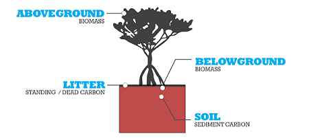
Figure 1. Three carbon pools for marine ecosystems included in the InVEST blue carbon model (mangrove example).

Note

Several parameters are shared across most of the equations in the model:

• \(t\) is the timestep. This model operates on an annual timescale, so \(t\) represents the year represented by the timestep.

  • \(t_{baseline}\) represents the year of the baseline landcover.

• \(s\) is the snapshot year. This represents the year of any of the transition snapshots after the baseline year.

• \(p\) represents the carbon pool, generally biomass or soil. The litter pool is considered only in the carbon accumulation calculations and is not affected by emissions.

The model considers each grid cell \(x\) independently, and has therefore been factored out of the equations described below.

Note

Although this user’s guide chapter refers to units in Megatonnes of CO2-equivalent per hectare, the model does no conversion of units whatsoever, and so any units representing the habitat-specific rate of accumulation or emissions, so long as they are consistent across all model inputs, may be used.

Carbon Storage

Coastal blue carbon habitats can simply indicate the dominant vegetation type (e.g., eelgrass, mangrove, etc), or they can be based on details that affect pool storage values such as plant species, vegetation density, temperature regime, or vegetation age (e.g., time since restoration or last major disturbance).

For the sake of the carbon storage estimation, each coastal blue carbon habitat is assumed to be in storage equilibrium at any point in time (accumulation of carbon will be accounted for in the sequestration component of the model).

Carbon stocks \(S\) for a given year \(t\) and pool \(p\) are calculated by adding the net carbon sequestration for year \(t\) to the stocks available in the prior year \(t-1\). Or, alternatively, by using the initial stock values from the biophysical table, \(S_{p,t_{baseline}}\).

(1)\[\begin{split}S_{p,t} = \begin{Bmatrix} S_{p,t-1} + N_{p,t} & if & t > t_{baseline} \\ S_{p,t_{baseline}} & if & t = t_{baseline} \end{Bmatrix}\end{split}\]

The carbon stocks for year \(t\) represent the carbon stocks at the very beginning of year \(t\).

Net sequestration \(N_{p,t}\) refers to the amount of carbon gained or lost within year \(t\), and the state of the most recent transition determines whether carbon is accumulating (positive net sequestration) or emitting (negative net sequestration). A single cell may either accumulate or emit carbon; it is not possible to do both within a single timestep. In this way, the model assumes that a grid cell transitions completely from one habitat type to another during a transition event. The nature of sequestration (accumulation or emission) will also remain consistent between transition years on a given pixel.

Therefore, \(N_{p,t}\) will be equal to one of these equations, depending on the state of the most recent transition:

(2)\[\begin{split}N_{p,t} = \begin{Bmatrix} -1 \cdot E_{p,t} & if & carbon\ is\ emitting \\ A_{p,t} & if & carbon\ is\ accumulating \end{Bmatrix}\end{split}\]

The rate of accumulation \(A_{p,t}\) is defined by the user in the biophysical table for each landcover classification. When a landcover class transitions into an accumulation state, the rate of accumulation will reflect the destination landcover class.

Note that emissions \(E_{p,t}\) is calculated as a positive value, and the \(-1\) is needed to reflect a loss of carbon from the pool.

Note that the above only applies to the biomass and soil pools. Litter stocks are not subject to emissions, and so may only accumulate linearly according to the rate defined by the user in the biophysical table:

(3)\[S_{p_{litter},t} = S_{p_{litter},t_{baseline}} + (A_{p_{litter}} \cdot (t - t_{baseline}))\]

Therefore, net sequestration for the litter pool, \(N_{p_{litter},t}\) is equivalent to \(A_{p_{litter}}\), which is defined by the user in the biophysical table. The rate of accumulation may change only when the landcover class transitions to another class.

The model also calculates total stocks for each timestep year \(t\), which is simply the sum of all carbon stocks in all 3 pools:

(4)\[S_{t,total} = S_{t,p_{soil}} + S_{t,p_{biomass}} + S_{t,p_{litter}}\]

Carbon Accumulation

We model accumulation as the rate of carbon retained in the soil in organic form after the first year of decomposition. In relation to the annual ecosystem budget, this pool has not been remineralized, so it represents net accumulation. This carbon is usually derived from belowground production, and residence time can range from decades to millennia (Romero et al. 1994, Mateo et al. 1997). This accumulation contributes to the development of carbon “reservoirs” which are considered virtually permanent unless disturbed. Thus, even in the absence of a land-use or land-cover change, carbon continues to be sequestered naturally.

Loss of carbon from the soil pool (sediments) upon disturbance is more nuanced than sequestration because different types of human uses and/or stasis may cause varied disruption of the soils and the carbon stored below. For example, high impact activities such as the clearing of mangroves for a shrimp pond or sediment dredging may result in a larger soil carbon disturbance than other activities such as commercial fishing or oil exploration. The impacts from coastal development on carbon storage vary since some types of development may involve paving over the soil, which often keeps a large percentage of the carbon stored intact. Alternatively, dredging could remove seagrasses and disturb the sediments below, releasing carbon into the atmosphere.

Carbon Emissions

When coastal ecosystems are degraded by human activities, the carbon stored in the living plant material (above and below the ground) and the soil may be emitted to the atmosphere. The magnitude of post-conversion CO₂ release depends on the type of vegetation disturbed and the level of disturbance. The type of disturbance will determine the amount of aboveground biomass loss and depth to which the soil profile will be altered. The deeper the effects of the disturbance, the more soil carbon that will be exposed to oxygen, oxidized and consequently emitted in the form of CO₂. Some disturbances will only disturb the top soil layers while the deeper layers remain inundated and their carbon intact. Other disturbances may affect several meters of the soil profile. To estimate the extent of the impact of various disturbances, we classify disturbances into three categories of impact: high, medium and low. Examples of high impact disturbances include mangrove conversion to shrimp farms and draining or diking salt marshes for conversion to agriculture. Low impact disturbance examples include recreational boating or float home marinas.

Carbon emissions begin in a snapshot year where the landcover classification underlying grid cell \(x\) transitions into a state of low-, med-, or high-impact disturbance. In subsequent years, emissions continue until either grid cell \(x\) experiences another transition, or else the analysis year is reached.

The model uses an exponential decay function based on the user-defined half-life \(H_{p}\) of the carbon pool in question, as well as the volume of disturbed carbon. In this case, \(s\) represents the year of the transition, and \(E_{p,t}\) is the volume of carbon emitted from pool \(p\) in year \(t\).

(5)\[E_{p,t} = D_{p,s} \cdot ({ 0.5 }^{ \frac { t-(s+1) }{ H_{p,s} } } - { 0.5 }^{ \frac { t-s }{ H_{p,s} } })\]

The volume of disturbed carbon \(D_{p,s}\) represents the total volume of carbon that will be released over time from the transition taking place on grid cell \(x\) in transition year \(s\) as time \(t \rightarrow \infty\). This quantity is determined by the magnitude of the disturbance \(M_{p,s}\) (low- med- or high-impact), the stocks \(S\) present at the beginning of year \(s\), and the landcover transition undergone in year \(s\):

(6)\[D_{p,s} = S_{p,s} \cdot M_{p,s}\]

The magnitude of the disturbance is determined by the transition matrix (low-, med-, or high-impact), and specified as a percentage of carbon disturbed in the Biophysical Table. When a landcover classification undergoes a transition into a state of emission, the disturbance magnitude will be taken from the source landcover class.

Magnitude and Timing of Loss

We model the release of carbon from the biomass and soil pools by estimating the fraction of carbon lost from each pool’s total stock at the time of disturbance. The fraction of carbon lost is determined by the original coastal blue carbon habitat and the level of impact resulting from the disturbance (see Table 1).

The InVEST Coastal Blue Carbon model allows users to provide details on the level of disturbance that occurs during a transition from a coastal blue carbon habitat to a non-coastal blue carbon habitat. This information can be provided to the model through a preprocessor tool and further clarified with an input transition table.

In general, carbon stock pools emit carbon at different rates: most emissions from the biomass pool take place within the first year, whereas emissions from the soil pool may take much longer. The model assigns exponential decay functions and half-life values to the biomass and soil carbon pools of each habitat type (Table 1; Murray et al. 2011).

Rank	Salt marshes	Mangroves	Seagrasses	Other vegetation
% carbon loss from biomass	LI/MI: 50% biomass loss (1) HI: 100% biomass loss	LI/MI: 50% biomass loss (1) HI: 100% biomass loss	LI/MI: 50% biomass loss (1) HI: 100% biomass loss	Use literature/field data
% carbon loss from soil	LI: 30% loss (1) MI/HI: 100% loss (3)	LI: 30% loss (1) MI: 50% loss (1) HI: 66% loss (up to 1.5 m depth) (1)	LI/MI: top 10% washes away, bottom 90% decomposes in place (2) HI: top 50% washes away, bottom 50% decomposes in place (2)	Use literature/field data
Rate of decay (over 25 years)	Biomass half-life: 6 months (2) Soil half-life: 7.5 years (2)	Biomass half-life: 15 years, but assume 75% is released immediately from burning Soil half-life 7.5 years (2)	Biomass half-life: 100 days (2) Soil half-life: 1 year (2)	Use literature/field data
Methane emissions	1.85 T CO2/ha/yr (4)	0.4 T CO2/ha/yr	Negligible	Use literature/field data

Table 1: Percent carbon loss and habitat-specific decay rates as a result of low (LI), medium (MI) and high (HI) impact activities disturbing salt marsh, mangrove, and seagrass ecosystems. These default values can be adjusted by modifying the input CSV tables.

References (numbers in parentheses above):

1. Donato, D. C., Kauffman, J. B., Murdiyarso, D., Kurnianto, S., Stidham, M., & Kanninen, M. (2011). Mangroves among the most carbon-rich forests in the tropics. Nature Geoscience, 4(5), 293-297.

2. Murray, B. C., Pendleton, L., Jenkins, W. A., & Sifleet, S. (2011). Green payments for blue carbon: Economic incentives for protecting threatened coastal habitats. Nicholas Institute for Environmental Policy Solutions, Report NI, 11, 04.

3. Crooks, S., Herr, D., Tamelander, J., Laffoley, D., & Vandever, J. (2011). Mitigating climate change through restoration and management of coastal wetlands and near-shore marine ecosystems: challenges and opportunities. Environment Department Paper, 121, 2011-009.

4. Krithika, K., Purvaja, R., & Ramesh, R. (2008). Fluxes of methane and nitrous oxide from an Indian mangrove. Current Science (00113891), 94(2).

Valuation of Net Sequestered Carbon

The valuation option for the blue carbon model estimates the economic value of sequestration (not storage) as a function of the amount of carbon sequestered, the monetary value of each ton of sequestered carbon, a discount rate, and the change in the value of carbon sequestration over time. The value of sequestered carbon is dependent on who is making the decision to change carbon emissions and falls into two categories: social and private. If changes in carbon emissions are due to public policy, such as zoning coastal areas for development, then decision-makers should weigh the benefits of development against the social losses from carbon emissions. Because local carbon emissions affect the atmosphere on a global scale, the social cost of carbon (SCC) is commonly calculated at a global scale (USIWGSCC, 2010). Efforts to calculate the social cost of carbon have relied on multiple integrated assessment models such as FUND (http://www.fund-model.org/), PAGE (Hope, 2011), DICE and RICE (https://sites.google.com/site/williamdnordhaus/dice-rice). The US Interagency Working Group on the Social Cost of Carbon has synthesized the results of some of these models and gives guidance for the appropriate SCC through time for three different discount rates (USIWGSCC, 2010; 2013). If your research questions lead you to a social cost of carbon approach, it is strongly recommended to consult this guidance. The most relevant considerations for applying SCC valuation based on the USIWGSCC approach in InVEST are the following:

• The discount rate that you choose for your application must be one of the three options in the report (2.5%, 3%, or 5%). In the context of policy analysis, discount rates reflect society’s time preferences. For a primer on social discount rates, see Baumol (1968).

• Since the damages incurred from carbon emissions occur beyond the date of their initial release into the atmosphere, the damages from emissions in any one period are the sum of future damages, discounted back to that point. For example, to calculate the SCC for emissions in 2030, the present value (in 2030) of the sum of future damages (2030 onward) is needed. This means that the SCC in any future period is a function of the discount rate, and therefore, a consistent discount rate should be used throughout the analysis. There are different SCC schedules (price list) for different discount rates. Your choice of an appropriate discount rate for your context will, therefore, determine the appropriate SCC schedule choice.

An alternative to SCC is the market value of carbon credits approach. If the decision-maker is a private entity, such as an individual or a corporation, they may be able to monetize their land use decisions via carbon credits. Markets for carbon are currently operating across several geographies and new markets are taking hold in Australia, California, and Quebec (World Bank, 2012). These markets set a cap on total emissions of carbon and require that emitters purchase carbon credits to offset any emissions. Conservation efforts that increase sequestration can be leveraged as a means to offset carbon emissions and therefore sequestered carbon can potentially be monetized at the price established in a carbon credit market. The means for monetizing carbon offsets depends critically on the specific rules of each market, and therefore it is important to determine whether or not your research context allows for the sale of sequestration credits into a carbon market. It is also important to note that the idiosyncrasies of market design drive carbon credit prices observed in the market and therefore prices do not necessarily reflect the social damages from carbon.

For further detail and discussion on the Social Cost of Carbon, refer to https://www.carbonbrief.org/qa-social-cost-carbon.

Net present value \(V\) is calculated for each snapshot year \(s\) after the baseline year, extending out to the final analysis year.

(7)\[V = \sum_{t=0}^{T} \frac{p_t (S_t - S_{t-1})}{(1+d)^t}\]

where

• \(V\) is the net present value of carbon sequestration

• \(T\) is the number of years between \(t_{baseline}\) and the snapshot year \(s\). If an analysis year is provided beyond the final snapshot year, this will be used in addition to the snapshot years.

• \(p_t\) is the price per ton of carbon at timestep \(t\)

• \(S_t\) represents the total carbon stock at timestep \(t\), summed across the soil and biomass pools.

• \(d\) is the discount rate

Note

The most recent carbon price table used for federal policy making in the United States can be found at https://www.epa.gov/sites/production/files/2016-12/documents/sc_co2_tsd_august_2016.pdf. For a discussion on why these methods are currently used in the US and what has happened since 2016, see the discussion at https://www.gao.gov/assets/710/707776.pdf.

The sample price tables that come with the latest version of InVEST are based on 2016 carbon price estimates from the US Environmental Protection Agency from the 2016 publication linked above. These tables are in USD from the year 2007, which is consistent with USIWGSCC estimates.

Identifying LULC Transitions with the Preprocessor

The land use / land cover (LULC) maps provide snapshots of a changing landscape and are the inputs that drive carbon accumulation and emissions in the model. The user must first produce a set of coastal and marine habitat maps via a land change model (e.g., SLAMM), a scenario assessment tool, or manual GIS processing. The user must then input the LULC maps into the model with an associated year so that the appropriate source and destination transitions may be determined.

The preprocessor tool compares LULC classes across the maps to identify the set of all LULC transitions that occur. The tool then generates a transition matrix that indicates whether a transition occurs between two habitats (e.g. salt marsh to developed dry land) and whether carbon accumulates, is disturbed, or remains unchanged once that transition occurs. The nature of carbon accumulation or disturbance is determined according to whether the landcover is transitioning to and/or from a coastal blue carbon habitat:

• Other LULC Class \(\Rightarrow\) Coastal Blue Carbon Habitat (Carbon Accumulation in Succeeding Years of Transition Event Until Next Bounding Year)

• Coastal Blue Carbon Habitat \(\Rightarrow\) Coastal Blue Carbon Habitat (Carbon Accumulation in Succeeding Years of Transition Event Until Next Bounding Year)

• Coastal Blue Carbon Habitat \(\Rightarrow\) Other LULC Class (Carbon Disturbance in Succeeding Years of Transition Event Until End of Time Series Forecast)

• Other LULC Class \(\Rightarrow\) Other LULC Class (No Carbon Change in Succeeding Years of Transition Event Until Next Bounding Year)

This transition matrix produced by the coastal blue carbon preprocessor, and subsequently edited by the user, allows the model to identify where human activities and natural events disturb carbon stored by vegetation. If a transition from one LULC class to another does not occur during any of the time steps, the cell will be left blank. For cells in the matrix where transitions occur, the tool will populate a cell with ‘accum’ in the cases where a non-coastal blue carbon habitat transitions to a coastal blue carbon habitat or a coastal blue carbon habitat transitions to another coastal blue carbon habitat, ‘disturb’ in the case where a coastal blue carbon habitat transitions to a non-coastal blue carbon habitat, or ‘NCC’ (for “no carbon change”) in the case where a non-coastal blue carbon habitat transitions to another non-coastal blue carbon habitat. For example, if a salt marsh pixel in \(s_{0}\) is converted to developed dry land in \(s_{1}\) then the cell will be populated with ‘disturb’. On the other hand, if a mangrove remains a mangrove over this same time period then this cell in the matrix will be populated with ‘accum’. It is likely that a mangrove that remains a mangrove will accumulate carbon in its soil and biomass.

The user will then need to modify the ‘disturb’ cells with either ‘low-impact-disturb’, ‘med-impact-disturb’ or ‘high-impact-disturb’ depending on the level of disturbance that occurs as the transition occurs between LULC types. This gives the user more fine-grained control over emissions due to disturbance. For example, rather than provide only one development type in an LULC map, a user can separate out the type into two development types and update the transition matrix accordingly so that the model can more accurately quantify and map changes in carbon as a result of natural and anthropogenic factors. Similarly, different species of mangroves may accumulate soil carbon at different rates. If this information is known, it can improve the accuracy of the model to provide this species distinction (two different classes in the LULC input maps) and then the associated accumulation rates in the Biophysical Table.

Limitations and Simplifications

In the absence of detailed knowledge on the dynamics of the carbon cycle in coastal and marine systems, we take the simplest accounting approach and draw on published carbon stock datasets from neighboring coastlines. We use carbon estimates from the most extensive and up-to-date published global datasets of carbon storage and accumulation rates (e.g., Fourqurean et al. 2012 & Silfeet et al. 2011).

• We assume all meaningful storage, accumulation and emission in case of impact occurs in the biomass and soil pools.

• We ignore increases in stock and accumulation with growth and aging of habitats.

• We assume that carbon is stored and accumulated linearly through time between transitions.

• We assume that, after a disturbance event occurs, the disturbed carbon is emitted over time at an exponential decay rate.

• We assume that some human activities that may degrade coastal ecosystems do not disturb carbon in the sediments.

• We assume that landcover transitions happen instantaneously and completely in the first moment of the year in which the transition occurs.

Data Needs and Running the Model

Because the Coastal Blue Carbon model relies upon the specific transitions from one landcover to another, an optional preprocessor has been provided to make it easier to identify the landcover transitions that take place on the lanscape and the nature of those transitions. The outputs of this preprocessor, if used, must then be edited by the user to indicate the magnitude of disturbances before being used as an input to the main model. The inputs for both the preprocessor and the main model are described here.

Please consult the InVEST sample data (located in the folder where InVEST is installed, if you also chose to install sample data) for examples of all of these data inputs. This will help with file type, folder structure and table formatting. Note that all GIS inputs must be in the same projected coordinate system and in linear meter units.

Step 1. Preprocessing - Coastal Blue Carbon Preprocessor

The preprocessor tool compares LULC classes across snapshot years in chronological order to identify the set of all LULC transitions that occur. From this set, the preprocessor generates a transition matrix that indicates whether a transition occurs between two habitats (e.g. salt marsh to developed dry land) and whether carbon accumulates, is disturbed, or remains unchanged once that transition occurs. It also produces a template biophysical table for the user to fill in with information quantifying carbon change due to LULC transitions. This table must be further edited by the user, and the edited table is a required input to the main Coastal Blue Carbon model. See the Identifying LULC Transitions with the Preprocessor section above for more information.

Inputs

• Workspace (required): The selected folder is used as the workspace where all intermediate and final output files will be written. If the selected folder does not exist, it will be created. If datasets already exist in the selected folder, they will be overwritten.

• Results suffix (optional): This text string will be appended to the end of the result file names to help distinguish outputs from multiple runs.

• LULC Snapshots Table (required): A CSV table mapping snapshot years to the location of GDAL-supported land use/land cover snapshot rasters. The pixel values of these rasters are unique integers representing each LULC class and must have matching code values in the LULC Lookup Table. The table format is as follows:

  snapshot_year	raster_path
  <int year>	<path>

  The path to rasters may be either absolute paths on this computer or paths relative to the location of the snapshots table itself.

• LULC Lookup Table (required): A CSV (.csv, Comma Separated Value) table used to map LULC classes to their values in a raster, as well as to indicate whether or not the LULC class is a coastal blue carbon habitat. The table format is as follows:

  lulc-class	code	is_coastal_blue_carbon_habitat
  <string>	<int>	<TRUE or FALSE>
  …	…	…

Where all columns are required and are defined as follows:

• lulc-class: Text string description of each land use/land cover (LULC) class

• code: Unique integer value for each LULC class. These integer values must match values in the user-supplied Land Use/Land Cover Rasters, and all LULC classes in the Land Use/Land Cover Rasters must be included in this LULC Lookup Table.

• is_coastal_blue_carbon_habitat: Enter a value of TRUE if the LULC type is coastal blue carbon habitat (e.g. mangroves, sea grass) and enter a value of FALSE if the LULC type is not blue carbon habitat (e.g. urban, agriculture.)

Outputs

Output files for the preprocessor are located in the folder Workspace/outputs_preprocessor. “Suffix” in the following file names refers to the optional user-defined Suffix input to the model.

• Parameter log: Each time the model is run, a text (.txt) file will be created in the main Workspace folder. The file will list the parameter values and output messages for that run and will be named according to the service, the date and time. When contacting NatCap about errors in a model run, please include this parameter log.

• transitions_[Suffix].csv: CSV (.csv, Comma Separated Value) format table, which is a transition matrix indicating whether disturbance or accumulation occurs in a transition from one LULC class to another. If the cell is left blank, then no transition of that kind occurs between the input Land Use/Land Cover Rasters. The left-most column (lulc-class) represents the source LULC class, and the top row (<lulc1>, <lulc2>…) represents the destination LULC classes. Depending on the transition type, a cell will be pre-populated with one of the following: empty if no such transition occurs, ‘NCC’ (for no carbon change), ‘accum’ (for accumulation) or ‘disturb’ (for disturbance). You must edit the ‘disturb’ cells with the degree to which disturbance occurs due to the LULC change. This is done by changing ‘disturb’ to either ‘low-impact-disturb’, ‘med-impact-disturb’, or ‘high-impact-disturb’.

The edited table is used as input to the main Coastal Blue Carbon model as the LULC Transition Effect of Carbon Table.

lulc-class	<lulc1>	<lulc2>	…
<lulc1>	<string>	<string>	…
<lulc2>	<string>	<string>	…
…	…	…	…

• carbon_pool_transient_template_[Suffix].csv: CSV (.csv, Comma Separated Value) format table, mapping each LULC type to impact and accumulation information. You must fill in all columns of this table except the ‘lulc-class’ and ‘code’ columns, which will be pre-populated by the model. See Step 2. The Main Model for more information. Accumulation units are (Megatonnes of CO₂ e/ha-yr), half-life is in integer years, and disturbance is in integer percent.

The edited table is used as input to the main Coastal Blue Carbon model as the Biophysical Table.

code	lulc-class	biomass-initial	soil-initial	litter-initial	biomass-half-life	biomass-low-impact-disturb	biomass-med-impact-disturb	biomass-high-impact-disturb	biomass-yearly-accumulation	soil-half-life	soil-low-impact-disturb	soil-med-impact-disturb	soil-high-impact-disturb	soil-yearly-accumulation	litter-yearly-accumulation
<int>	<lulc1>
<int>	<lulc2>
…	…

• aligned_lulc_[year]_[Suffix].tif: Rasters that are the result of aligning all of the input LULC rasters with each other. All rasters are resampled to the minimum resolution of the input rasters and cropped to the intersection of their bounding boxes. Any resampling needed is done using nearest-neighbor interpolation. You generally don’t need to do anything with these files.

Step 2. The Main Model - Coastal Blue Carbon

The main Coastal Blue Carbon model calculates carbon stock and sequestration over time, based on the transition and carbon pool information generated by the preprocessor and edited by the user. It can also calculate the value of sequestration if economic data is provided.

Inputs

• Workspace (required): The selected folder is used as the workspace where all intermediate and final output files will be written. If the selected folder does not exist, it will be created. If datasets already exist in the selected folder, they will be overwritten.

• Results suffix (optional): This text string will be appended to the end of the result file names to help distinguish outputs from multiple runs.

• Biophysical Table (required): A table identifying landcover classes and codes represented in the snapshot LULC rasters and relating these codes to the initial quantities of carbon, rates of accumulation and magnitudes of disturbance in each carbon pool. A template of this table is produced by the preprocessor (described above), and is also included with the sample data for the model.

  The columns required in this table are:

  • lulc-class - the textual representation of the landcover classification. This label must be unique among the landcover classifications.

  • code - The integer landcover code used in the LULC snapshot rasters to represent this landcover class.

  • biomass-initial - the initial carbon stocks (megatonnes CO2E per hectare) in the biomass pool for this landcover classification.

  • soil-initial - the initial carbon stocks (megatonnes CO2E per hectare) in the soil pool for this landcover classification.

  • litter-initial - the initial carbon stocks (megatonnes CO2E per hectare) in the litter pool for this landcover classification.

  • biomass-half-life - the half-life (in years) of the carbon stored in the biomass pool. This must be a numeric value greater than 0.

  • biomass-low-impact-disturb - the decimal (0-1) percentage of the carbon stock in the biomass pool that is disturbed when a cell transitions away from this landcover classification in a low-impact disturbance event.

  • biomass-med-impact-disturb - the decimal (0-1) percentage of the carbon stock in the biomass pool that is disturbed when a cell transitions away from this landcover classification in a medium-impact disturbance event.

  • biomass-high-impact-disturb - the decimal (0-1) percentage of the carbon stock in the biomass pool that is disturbed when a cell transitions away from this landcover classification in a high-impact disturbance event.

  • biomass-yearly-accumulation - the annual rate of accumulation (megatonnes CO2E per hectare) in the biomass pool.

  • soil-half-life - the half-life (in years) of the carbon stored in the soil pool. This must be a numeric value greater than 0.

  • soil-low-impact-disturb - the decimal (0-1) percentage of the carbon stock in the soil pool that is disturbed when a cell transitions away from this landcover classification in a low-impact disturbance event.

  • soil-med-impact-disturb - the decimal (0-1) percentage of the carbon stock in the soil pool that is disturbed when a cell transitions away from this landcover classification in a medium-impact disturbance event.

  • soil-high-impact-disturb - the decimal (0-1) percentage of the carbon stock in the soil pool that is disturbed when a cell transitions away from this landcover classification in a high-impact disturbance event.

  • soil-yearly-accumulation - the annual rate of accumulation (megatonnes CO2E per hectare) in the soil pool.

  • litter-annual-accumulation - the annual rate of accumulation (megatonnes CO2E per hectare) in the litter pool. This will generally be 0.0, but can be adjusted if needed.

• Landcover Transitions Table (required): CSV (.csv, Comma Separated Value) table, based on the transitions_[Suffix].csv table generated by the preprocessor. You must edit transitions_[Suffix].csv as described in Step 1 Preprocessing Outputs before it can be used by the main model. The left-most column (lulc-class) represents the source LULC class, and the top row (<lulc1>, <lulc2>…) represents the LULC classes that it transitions to. The classes represented in this table must exactly match the classes (in the lulc-class column) defined in the biophysical table.

  lulc-class	<lulc1>	<lulc2>	…
  <lulc1>	<str>	<str>	…
  <lulc2>	<str>	<str>	…
  …	…	…	…

• Landcover Snapshots Table (required): A CSV table containing paths to the land-use / land cover rasters of each snapshot year and the year the snapshot raster represents. The raster with the earliest chronological year will be used as the baseline raster. If rasters provided in this table have different extents or resolutions, they will be resampled to the minimum resolution of the set of rasters, and clipped to the intersection of all of the bounding boxes.

  If you are only interested in the standing stock of carbon at a single year, then only provide a single row in this table.

  These rows may be provided in any order desired.

  All rasters provided in this table must be in a projected coordinate system with units in meters.

  Required columns:

  • snapshot_year - the integer year that the raster in this row represents. Each snapshot year must be unique in this table; the same snapshot year cannot be provided twice.

  • raster_path - the path to a landcover raster on disk. May be an absolute path, or relative to the location of this CSV file on disk. The raster located at this path must be a land-use / land cover raster with integer codes matching those in the biophysical table.

• Analysis Year (optional): An integer year value that may be used to extend the analysis for longer than the Snapshot Years. For example, carbon will continue to accumulate or emit after the last Snapshot Year, until the Analysis Year. This value must be further in the future than the final LULC transition (“snapshot”) year.

• Calculate Net Present Value of Sequestered Carbon (optional): If you want the model to calculate the monetary value of sequestration, check this box. You have the choice to model the value of carbon sequestration using a price schedule (using the input Price Table), or by supplying a base year carbon price (input Price) and an annual rate of interest (input Interest Rate). In both cases, an appropriate discount rate is necessary.

The value of carbon sequestration over time is given by:

• Value of a sequestered ton of carbon: This user’s guide assumes carbon is measured in tons of CO₂. If you have prices in terms of tons of elemental carbon, these need to be converted to prices per ton of CO₂. This requires dividing the price by a factor of 3.67 to reflect the difference in the atomic mass between CO₂ and elemental carbon. Again, this value can be input using a price schedule over the appropriate time horizon, or by supplying a base year carbon price and an annual rate of inflation.

• Discount rate: (\(d\) in the net present value equation), which reflects time preferences for immediate benefits over future benefits. If the rate is set equal to 0% then monetary values are not discounted.

If the Calculate Net Present Value of Sequestered Carbon box is checked, you must also provide the following valuation information.

• Use Price Table (optional): If you want to provide a table of carbon prices for different years, check this box. If the box is checked, you must also provide the Price Table input.

• Price (required for valuation if Price Table is not used): The price per Megatonne CO₂ e at the baseline year. Floating point value, may be in any currency.

• Interest Rate (required for valuation if Price Table is not used): The interest rate on the price per Megatonne CO₂ e, compounded yearly. Floating point percentage (%) value. For example, an interest rate of 3% would be entered as “3”.

• Price Table (optional): CSV (.csv, Comma Separated Value) table that can be used in place of the Price and Interest Rate inputs. This table contains the price per Megatonne CO₂ e sequestered for a given year, for all years from the original Snapshot Year to the Analysis Year, if provided. Year is an integer value; price is a floating point value, may be in any currency, but must be in the same currency for all years.

  year	price
  <int>	<float>
  <int>	<float>
  …	…

• Discount Rate (required): The discount rate on future valuations of sequestered carbon, compounded yearly. Floating point value.

Outputs

The output files for the main Coastal Blue Carbon model are located in the folder Workspace/outputs, and intermediate files in Workspace/intermediate. “Suffix” in the following file names refers to the optional user-defined Suffix input to the model.

• Parameter log: Each time the model is run, a text (.txt) file will be created in the main Workspace folder. The file will list the parameter values and output messages for that run and will be named according to the service, the date and time. When contacting NatCap about errors in a model run, please include this parameter log.

Workspace/outputs

• carbon-accumulation-between-[year]-and-[year][Suffix].tif. Amount of carbon accumulated between the two specified years. Units: Megatonnes CO₂ e per Hectare

• carbon-emissions-between-[year]-and-[year][Suffix].tif. Amount of carbon lost to disturbance between the two specified years. Units: Megatonnes CO₂ e per Hectare

• carbon-stock-at-[year][Suffix].tif. Sum of the 3 carbon pools for each LULC for the specified year. Units: Megatonnes CO₂ e per Hectare

• total-net-carbon-sequestion-between-[year]-and-[year][Suffix].tif. Total carbon sequestration between the two specified years, based on accumulation minus emissions during that time period. Units: Megatonnes CO₂ e per Hectare

• total-net-carbon-sequestration[Suffix].tif. Total carbon sequestration over the whole time period between the Baseline and either the latest Snapshot Year or the Analysis Year, based on accumulation minus emissions. Units: Megatonnes CO₂ e per Hectare

• net-present-value[Suffix].tif. Monetary value of carbon sequestration. Units: (Currency of provided Prices) per Hectare

Workspace/intermediate

This folder contains input rasters that have all been resampled and aligned to the same bounding box, as intermediate steps in the modeling process. Generally, you don’t need to do anything with these files.

• stocks-[pool]-[year][suffix].tif - the carbon stocks available at the Beginning of the year noted in the filename. Units: Megatonnes CO2E per hectare

• accumulation-[pool]-[year][suffix].tif - the spatial distribution of rates of carbon accumulation in the given pool at the given year. Years will represent the snapshot years in which the accumulation raster takes effect. Units: Megatonnes CO2E per hectare.

• halflife-[pool]-[year][suffix].tif - a raster of the spatial distribution of the half-lives of carbon in the pool mentioned at the given snapshot year. Units: years.

• disturbance-magnitude-[pool]-[year][suffix].tif - the magnitude of disturbance in the given pool in the given snapshot year. Units: 0-1, the percentage of carbon disturbed.

• disturbance-volume-[pool]-[year][suffix].tif - the volume of the carbon disturbed in the snapshot year. This is a function of the carbon stocks at the year prior and the disturbance magnitude in the given snapshot year. See cbc_disturbance_volume Units: Megatonnes CO2E per hectare.

• year-of-latest-disturbance-[pool]-[year][suffix].tif - each cell indicates the most recent year in which the cell underwent a landcover transition.

• aligned-lulc-[snapshot type]-[year][suffix].tif - the snapshot landcover raster of the given year, aligned to the intersection of the bounding boxes of all snapshot rasters, and with consistent cell sizes. The cell size of the aligned landcover rasters is the minimum of the incoming cell sizes.

• net-sequestration-[pool]-[year][suffix].tif - the net sequestration in the given pool in the given year. See (2) Units: Megatonnes CO2E per hectare.

• total-carbon-stocks-[year][suffix].tif - the sum of the stocks present across all three carbon pool at the given year. Units: Megatonnes CO2E per Hectare.

Advanced Usage: Spatially-explicit Biophysical Parameters

While the Coastal Blue Carbon’s preprocessor and main model user interfaces are helpful for most cases that can be classified into various landcover types, an advanced user may desire to provide spatially explicit maps of carbon half-lives, rates of accumulation, and other biophysical parameters to the model. This is not possible through the User Interface, but is available as a python function that provides lower-level access to the model’s timeseries analysis. Use of this advanced functionality requires a substantial amount of data preprocessing and has much more complex data requirements. Please see the model’s source code on github for details: https://github.com/natcap/invest/blob/main/src/natcap/invest/coastal_blue_carbon/coastal_blue_carbon.py

Example Use-Case

Freeport, Texas

Summary

Over the next 100 years, the US Gulf coast has been identified as susceptible to rising sea levels. The use of the InVEST blue carbon model serves to identify potential changes in the standing stock of carbon in coastal vegetation that sequester carbon. This approach in Freeport, TX was made possible with rich and resolute elevation and LULC datasets. We used a 10-meter DEM with sub-meter vertical accuracy to model marsh migration and loss over time as a result of sea level rise (SLR) using Warren Pinnacle’s SLAMM (Sea Level Affected Marsh Model). Outputs from SLAMM serve as inputs to the InVEST Coastal Blue Carbon model which permits the tool to map, measure, and value carbon sequestration and emissions resulting from changes to coastal land cover over a 94-year period.

The Sea Level Affecting Marshes Model (SLAMM: http://www.warrenpinnacle.com/prof/SLAMM/) models changes in the distribution of 27 different coastal wetland habitat types in response to sea-level rise. The model relies on the relationship between tidal elevation and coastal wetland habitat type, coupled with information on slope, land use, erosion and accretion to predict changes or loss of habitat. SLAMM outputs future habitat maps for user-defined time steps and sea-level rise scenarios. These future habitat maps can be utilized with InVEST service models to evaluate resultant changes in ecosystem services under various sea-level rise scenarios (e.g. 1 meter SLR by 2100).

For example, SLAMM was used to quantify differences in carbon sequestration over a range of sea-level rise projections in Galveston Bay, Texas, USA. First, SLAMM was used to map changes in the distribution of coastal wetland habitat over time under different sea-level rise projections. Then, the InVEST Coastal Blue Carbon model was used to evaluate changes in carbon sequestration associated with predicted changes in habitat type. The 27 land-cover classes modeled by SLAMM were condensed into a subset relevant to carbon sequestration and converted from ASCII to raster format for use with InVEST. SLAMM results produced LULC maps of future alternative scenarios over 25-year time slices beginning in 2006 and ending in 2100. The following figure depicts 2006 LULC and a table of disaggregated land class types.

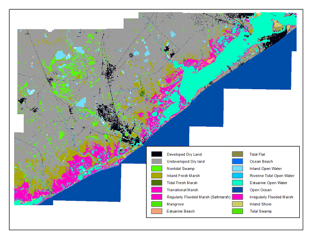
Figure CS1. Current (2006) LULC map of Freeport, Texas

Carbon stored in the sediment (‘soil’ pool) was the focus of this analysis. The vast majority of carbon is sequestered in this pool by coastal and marine vegetation. See the case study limitations for additional information. To produce maps of carbon storage at the different 25-year time steps, we used the model to perform a simple “look-up” to determine the amount of carbon per 10-by-10 meter pixel based on known storage rates from sampling in the Freeport area (Chmura et al. 2003).

Next, we provide the InVEST model with a transition matrix in order to identify the amount of carbon gained or lost over each 25-year time step. Annual accumulation rates in the salt marsh were also obtained from Chmura et al. (2003). When analyzing the time period from 2025 to 2050, we assume \(t_{2}\) = 2025 and \(t_{3}\) = 2050. We identify all the possible transitions that will result in either accumulation or loss of carbon. The model compares the two LULC maps (\(t_{2}\) and \(t_{3}\)) to identify any pixel transitions from one land cover type to another. We apply these transformations to the standing stock of carbon which is the running carbon tally at \(t_{2}\) (2025). Once these adjustments are complete, we have a new map of standing carbon for \(t_{3}\) (2050). We repeat this step for the next time period where \(t_{3}\) = 2050 and \(t_{4}\) = 2075. This process was repeated until 2100. The model produces spatially explicit depictions of net sequestration over time as well as summaries of net gain/emission of carbon for the two scenarios at each 25-year time step. This information was used to determine during which time period for each scenario the rising seas and resulting marsh migration led to net emissions for the study site and the entire Freeport area.

Time Period	Scenario #1: No Management	Scenario #2: High Green
2006-2025 (\(t_{1}\)-\(t_{2}\))	+4,031,180	+4,172,370
2025-2050 (\(t_{2}\)-\(t_{3}\))	-1,170,580	+684,276
2050-2075 (\(t_{3}\)-\(t_{4}\))	-7,403,690	-5,525,100
2075-2100 (\(t_{4}\)-\(t_{5}\))	-7,609,020	-8,663,600
100-Year Total:	-12,152,100	-9,332,050

Table CS1. Carbon sequestration and emissions for each 25-year time period for the two scenarios of the entire Freeport study area.

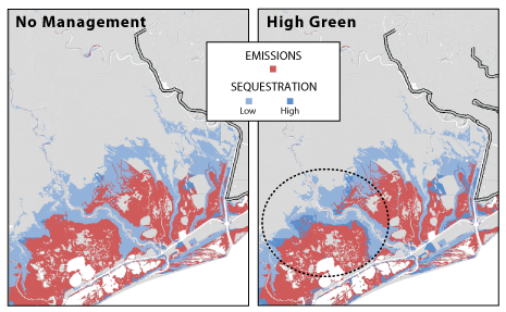
Figure CS2. Carbon emissions (red) and sequestration (blue) from 2006 to 2100 for the two scenarios and a subset of the Freeport study area.

The following is table summarizing how the main inputs, where they were obtained and how they were used in the model:

Input	Source	Use in the InVEST blue carbon model
DEM	USGS	DEM was needed to produce the future LULC maps using the SLAMM tool.
Land use / land cover (LULC)	USGS/NOAA	Salt marshes store carbon in biomass and soils. We utilized maps showing the current distribution of salt marshes to establish a baseline coverage of marshes from which we estimate aboveground biomass and soil carbon.
Carbon stock in salt marsh systems	Natural Capital Project literature review	Carbon storage was calculated by summing the carbon stored in biomass and sediments. Carbon stocks were calculated for all of the areas of functional salt marsh in the study region (Chmura et al. 2003).
Social value of carbon in 2006 US $	USIWGSCC 2010	The “social cost of carbon” (SCC) is an estimate of the monetized damages associated with an incremental increase in carbon emissions in a given year. It is intended to include (but is not limited to) changes in net agricultural productivity, human health, property damages from increased flood risk, and the value of ecosystem services. The social cost of carbon is useful for allowing institutions to incorporate the social benefits of reducing carbon dioxide (CO2) emissions into cost benefit analyses of management actions that have small, or “marginal,” impacts on cumulative global emissions.
Discount rate	USIWGSCC 2010	This discount rate reflects society’s preferences for short run versus long term consumption. Since carbon dioxide emissions are long-lived, subsequent damages occur over many years. We use the discount rate to adjust the stream of future damages to its present value in the year when the emissions were changed.

Table CS2. Input summary table for using InVEST blue carbon model in Freeport, Texas

Limitations

• This analysis did not model change in carbon resulting from growth or loss of aboveground biomass of coastal and marine vegetation.

• While the spatial resolution of the LULC maps produced by SLAMM was very high (10 meters), the temporal resolution provided by SLAMM was quite coarse (25-year time steps). The carbon cycle is a dynamic process. By analyzing change over 25-year time periods, we ignore any changes that are not present at the start and end of each time step.

References

Baumol, W. J. (1968). On the social rate of discount. The American Economic Review, 788-802.

Bouillon, S., Borges, A. V., Castañeda-Moya, E., Diele, K., Dittmar, T., Duke, N. C., … & Twilley, R. R. (2008). Mangrove production and carbon sinks: a revision of global budget estimates. Global Biogeochemical Cycles, 22(2).

Chmura, G. L., Anisfeld, S. C., Cahoon, D. R., & Lynch, J. C. (2003). Global carbon sequestration in tidal, saline wetland soils. Global biogeochemical cycles, 17(4).

Clough, J. S., Park, R., and Fuller, R. (2010). “SLAMM 6 beta Technical Documentation.” Available at http://warrenpinnacle.com/prof/SLAMM.

Fourqurean, J. W., Duarte, C. M., Kennedy, H., Marbà, N., Holmer, M., Mateo, M. A., … & Serrano, O. (2012). Seagrass ecosystems as a globally significant carbon stock. Nature Geoscience, 5(7), 505-509.

Hope, Chris. (2011) “The PAGE09 Integrated Assessment Model: A Technical Description.” Cambridge Judge Business School Working Paper No. 4/2011 (April). Available at https://www.jbs.cam.ac.uk/fileadmin/user_upload/research/workingpapers/wp1104.pdf.

Houghton, R. A. (2003). Revised estimates of the annual net flux of carbon to the atmosphere from changes in land use and land management 1850–2000. Tellus B, 55(2), 378-390.

Pendleton, L., Donato, D. C., Murray, B. C., Crooks, S., Jenkins, W. A., Sifleet, S., … & Baldera, A. (2012). Estimating global “blue carbon” emissions from conversion and degradation of vegetated coastal ecosystems. PLoS One, 7(9), e43542.

Rosenthal, A., Arkema, K., Verutes, G., Bood, N., Cantor, D., Fish, M., Griffin, R., and Panuncio, M. (In press). Identification and valuation of adaptation options in coastal-marine ecosystems: Test case from Placencia, Belize. Washington, DC: InterAmerican Development Bank. Technical Report.

Sifleet, S., Pendleton, L., and B. Murray. (2011). State of the Science on Coastal Blue Carbon. Nicholas Institute Report, 1-43.

United States, Interagency Working Group on Social Costs of Carbon. (2010) “Technical Support Document: Social Cost of Carbon for Regulatory Impact Analysis Under Executive Order 12866.” Available at https://www.epa.gov/sites/production/files/2016-12/documents/scc_tsd_2010.pdf.

United States, Interagency Working Group on Social Costs of Carbon. (2013) “Technical Update of the Social Cost of Carbon for Regulatory Impact Analysis Under Executive Order 12866.” Available at https://environblog.jenner.com/files/technical-update-of-the-social-cost-of-carbon-for-regulatory-impact-analysis-under-executive-order-12866.pdf.

World Bank. (2012). State and Trends of the Carbon Market 2012. Washington DC: The World Bank, 133.