Coastal Vulnerability Model

Summary

Faced with an intensification of human activities and a changing climate, coastal communities need to better understand how modifications of the biological and physical environment (i.e. direct and indirect removal of natural habitats for coastal development) can affect their exposure to storm-induced erosion and flooding (inundation). The InVEST Coastal Vulnerability model produces a qualitative estimate of such exposure in terms of a vulnerability index, which differentiates areas with relatively high or low exposure to erosion and inundation during storms. By coupling these results with global population information, the model can show areas along a given coastline where humans are most vulnerable to storm waves and surge. The model does not take into account coastal processes that are unique to a region, nor does it predict long- or short-term changes in shoreline position or configuration.

Model inputs, which serve as proxies for various complex shoreline processes that influence exposure to erosion and inundation, include: a polyline with attributes about local coastal geomorphology along the shoreline, polygons representing the location of natural habitats (e.g., seagrass, kelp, wetlands, etc.), rates of (observed) net sea-level change, a depth contour that can be used as an indicator for surge level (the default contour is the edge of the continental shelf), a digital elevation model (DEM) representing the topography of the coastal area, a point shapefile containing values of observed storm wind speed and wave power, and a raster representing population distribution.

Outputs can be used to better understand the relative contributions of these different model variables to coastal exposure and highlight the protective services offered by natural habitats to coastal populations. This information can help coastal managers, planners, landowners and other stakeholders identify regions of greater risk to coastal hazards, which can in turn better inform development strategies and permitting. The results provide a qualitative representation of coastal hazard risks rather than quantifying shoreline retreat or inundation limits.

Introduction

Coastal regions, which are constantly subject to the action of ocean waves and storms, naturally experience erosion and inundation over various temporal and spatial scales. However, coastal erosion and inundation pose a threat to human populations, activities and infrastructure, especially within the context of a changing climate and increasing coastal populations. Moreover, these increases in anthropogenic pressure can lead to the loss and degradation of coastal ecosystems and their ability to provide protection for humans during storms. Thus, it is important to understand the role of various biological and geophysical factors in increasing or decreasing the threat of coastal erosion and inundation in order to better plan for future development. In particular, it is important to know how natural habitats can mitigate the forces responsible for coastal erosion and inundation so that management actions might best preserve the protective services provided by coastal ecosystems.

A number of models estimate the vulnerability of coastal regions to long-term sea level rise, erosion and inundation based on geophysical characteristics (Gornitz et al. 1991, Hammar-Klose and Thieler 2001, Cooper and McLaughlin 1998). There are also methods to qualitatively estimate the relative role natural habitats play in reducing the risk of erosion and inundation of particular areas (WRI 2009, Bush et al. 2001). However, few models map the relative vulnerability of coastal areas to erosion and inundation based on both the geophysical and natural habitat characteristics of a region. It is our aim to fill that gap with the Coastal Vulnerability model.

The Coastal Vulnerability model produces a qualitative index of coastal exposure to erosion and inundation as well as summaries of human population density in proximity to the coastline. The model does not value directly any ecoystem service, but ranks sites as having a relatively low, moderate or high risk of erosion and inundation. It is relatively simple to use and quick to run, and it can be applied in most regions of the world with data that are, for the most part, relatively easy to obtain.

Model outputs are geospatial datasets, with a spatial resolution defined by the modeler, and can be overlaid with other spatial information for users to perform further analysis as they see fit. By highlighting the relative role of natural habitat at reducing exposure and showing the areas where coastal populations are threatened, the model can be used to investigate how some management action or land use change can affect the exposure of human populations to erosion and inundation.

The Model

The InVEST Coastal Vulnerability model produces an exposure index rank for each point along a coastline at an interval specified by the user. The exposure index represents the relative exposure of different coastline segments to erosion and inundation caused by storms within the region of interest. The coastal population raster shows the distribution of human population density within the coastal region of interest. The index is constructed using up to seven bio-geophysical variables. These variables represent the variations in natural biological and geomorphic characteristics across the region, the rate or amount of sea-level rise, the local bathymetry and topography, and the relative wind and wave forcing associated with storms. The model assesses the exposure of each shore segment within the domain of interest, relative to all other shore segments. Model outputs are potentially relevant at a variety of scales and extents, depending on the resolution of the input data. The model is suitable for wide, exposed, uniform coastlines and for complex, heterogenous, sheltered coastlines. Finally, the model also summarizes the coastal population density at the same scale as the exposure index, which can be used to create maps that show the relative vulnerability of human populations to coastal storms.

How it Works

The model calculates the exposure index and coastal population density using a spatial representation of the following bio-geophysical variables:

1. Relief

2. Natural habitats (biotic and abiotic)

3. Wind Exposure

4. Wave Exposure

5. Surge potential depth contour

6. Geomorphology (optional)

7. Sea level change (optional)

The primary output of the model is a geospatial dataset (points) that are plotted at user-defined interval along the shoreline in the coastal region of interest. This point dataset includes a table with a number of indices and rankings of input variables (described below) and can be used to the create maps that fit the user’s needs. Below are details describing the model variables and how the outputs are created.

Exposure Index

The model computes the coastal exposure index by combining the ranks of up to seven biological and physical variables at each shoreline point. Ranks vary from very low exposure (rank=1) to very high exposure (rank=5), based on a mixture of user- and model-defined criteria. This ranking system is based on methods proposed by Gornitz et al. (1990) and Hammar-Klose and Thieler (2001).

Table 1 Example Ranking Table

Rank	1 (very low)	2 (low)	3 (moderate)	4 (high)	5 (very high)
Geomorphology	Rocky; high cliffs; fjord; fiard; seawalls	Medium cliff; indented coast; bulkheads and small seawalls	Low cliff; glacial drift; alluvial plain; revetments; rip-rap walls	Cobble beach; estuary; lagoon; bluff	Barrier beach; sand beach; mud flat; delta
Relief	81 to 100 Percentile	61 to 80 Percentile	41 to 60 Percentile	21 to 40 Percentile	0 to 20 Percentile
Natural Habitats	Coral reef; mangrove; coastal forest	High dune; marsh	Low dune	Seagrass; kelp	No habitat
Sea Level Change	0 to 20 Percentile	21 to 40 Percentile	41 to 60 Percentile	61 to 80 Percentile	81 to 100 Percentile
Wave Exposure	0 to 20 Percentile	21 to 40 Percentile	41 to 60 Percentile	61 to 80 Percentile	81 to 100 Percentile
Surge Potential	0 to 20 Percentile	21 to 40 Percentile	41 to 60 Percentile	61 to 80 Percentile	81 to 100 Percentile

The model calculates the exposure index \(EI\) for each shoreline point as the geometric mean of all the variable ranks:

(113)\[EI = \left ({R_{Geomorphology} R_{Relief} R_{Habitats} R_{SLR} R_{WindExposure} R_{WaveExposure} R_{Surge}} \right )^{1/7}\]

or more generally:

(114)\[EI = \left (\prod_{i=1}^{n}R_i \right )^{1/n}\]

where \(R_i\) represents the ranking of the \(i^{th}\) bio-geophysical variable to calculate \(EI\).

Additionally, we provide tabular output of all intermediate results computed by the model so users can, for example, compute an \(EI\) using a different subset of \(R\) variables, or even a different equation.

In the remainder of this section, we first describe how the area of interest and shoreline points are defined, and then we provide a more detailed description of the variables presented in Example Ranking Table.

Shore Points and Area of Interest

Users can model coastal exposure at any scale and for any coastline on the globe within latitudes -65 degrees south and 77 degrees north (see Wind Exposure for details on this limitation). The model requires a polygon vector representing landmasses within the area of interest. From this landmass, the model plots points along the coastline at a distance interval specified by the user as the model resolution. For all the variables described in sections below, the model assigns a value for each shore point. Model runtime is highly dependent on the level of detail in the landmass polygon, which along with the model resolution, influences the number of total shoreline points.

Shore points will be plotted along all line segments of the landmass polygon that are within the area of interest polygon. Users may wish to exclude small uninhabited offshore features where it does not make sense to evaulate coastal hazard exposure. Such features will still be present for processes that assess wind and wave exposure to the other shore points.

Geomorphology

Rocky cliffs are less prone to erosion and inundation than bluffs, beaches or deltas. Consequently, a relative ranking of exposure scheme based on geomorphology similar to the one proposed by Hammar-Klose and Thieler (2001) has been adopted. Supplied in Appendix A is a definition of the terms used in this classification, which applies mostly to the North American continent.

The Geomorphology input should be a polyline vector with segments that categorize – in an attribute field called ‘RANK’ – the shoreline geomorphology based on the scheme presented in Example Ranking Table. The model joins the geomorphology ranks to shore points by searching around each point with a radius of half the model resolution and then taking the average of all the ranks found in the search. If no geomorphology segments are found in the search, the rank chosen for geomorphology fill value is assigned to the point. In this instance the shore points that received the geomorphology fill value are saved to an intermediate output file (intermediate/geomorphology/shore_points_missing_geomorphology.gpkg) for convenience. If very many points are missing data, it might be explained by spatial inaccuracy of either the geomorphology or landmass polygon inputs. Editing the geometory of one or both in GIS could help resolve this.

If the user’s geomorphology data source has more categories than the ones presented in Example Ranking Table, it is left to the user’s discretion to reclassify their data to match the provided ranking system, as explained in the Data Needs section, and in Appendix B.

It is recommend that the user include shore parallel hard structures (seawalls, bulkheads, etc.) in this classification and that they apply a low to moderate rank (1-3), depending on their characteristics. For example, a large, concrete seawall should be assigned a rank 1 as they are typically designed to prevent inundation during storm events and are designed to withstand damage or failure during the most powerful storms. It is recommended that low revetments or riprap walls be assigned a rank of 3 as they do not prevent inundation and may fail during extreme events.

The ranking presented in the above table is only a suggestion. Users should change the ranking of different shoreline types as they see fit, based on local research and knowledge, and by following directions presented in the Data Needs section.

Relief

Sites that are, on average, at greater elevations above Mean Seal Level (MSL) are at a lower risk of being inundated than areas at lower elevations. Relief is defined in the model as the average elevation of the coastal land area that is within a user-defined elevation averaging radius around each shore point. For this variable, the model requires a Digital Elevation Model (DEM) that covers the area of interest and extends beyond the AOI by at least the distance of the elevation averaging radius.

If there are no valid DEM pixels within the search radius of a shore point, that point will not receive a relief rank and the final Exposure Index at that point will not be calculated since a key variable (R_relief) of equation (113) is missing. These missing values will be evident in the coastal_exposure.csv and intermediate_exposure.csv output files. If there are many missing values, users may wish to increase the elevation averaging radius or confirm that the DEM and landmass polygon inputs are well aligned with each other.

Natural Habitats

Natural habitats (marshes, seagrass beds, mangroves, coastal dunes, or others) play a vital role in decreasing the impacts of coastal hazards that can erode shorelines and harm coastal communities. For example, large waves break on coral reefs before reaching the shoreline, mangroves and coastal forests dramatically reduce wave heights in shallow waters, and decrease the strength of wave- and wind-generated currents, seagrass beds and marshes stabilize sediments and encourage the accretion of nearshore beds as well as dissipate wave energy. On the other hand, beaches with little to no biological habitats or sand dunes offer little protection against erosion and inundation.

To compute a Natural Habitat exposure rank for a given shoreline point, the model determines whether a certain class of natural habitat (Example Ranking Table) is within a user-defined search radius from the point. (See Section 2 and Appendix B for a description of how the model processes natural habitat input layers.) When all \(N\) habitats in proximity to that point have been identified, the model creates an array R that contains all the ranks \(R_{k}, 1 \le k \le N\), associated with these habitats, as defined in Example Ranking Table. Using those rank values, the model computes a final Natural Habitat exposure rank for that point with the following formula:

(115)\[R_{Hab} = 4.8-0.5 \sqrt{ ( 1.5 \max_{k=1}^N (5-R_k) )^2 + \sum_{k=1}^N (5-R_k)^2 - (\max_{k=1}^N (5-R_k) )^2}\]

where the habitat that has the lowest rank is weighted 1.5 times higher than all other habitats that are present near a segment. This formulation allows us to maximize the accounting of the protection services provided by all natural habitats that front a shoreline segment. In other words, it ensures that segments that are fronted or have only one type of habitat (e.g., high sand dune) are more exposed than segments with more than one habitat (e.g., coral reefs and high sand dune). See Appendix B for a detailed account of all possible final rank values that can be obtained with equation (115).

To include this variable in the exposure index calculation, the model requires separate polygon shapefiles representing each natural habitat type, the rank, or level of protection offered by the habitat, and a protection distance, beyond which the habitat does not protect the coastline. All of these parameters are specified in the Habitats Table (CSV) (see Habitats Table section under Data Needs).

The ranking proposed in Example Ranking Table is based on the fact that fixed and stiff habitats that penetrate the water column (e.g., coral reefs, mangroves) and sand dunes are the most effective in protecting coastal communities. Flexible and seasonal habitats, such as seagrass, reduce flows when they can withstand their force, and encourage accretion of sediments. Therefore, these habitats receive a lower ranking than fixed habitats. It is left to the user’s discretion to separate sand dunes into high and low categories. It is suggested, however, that since category 4 hurricanes can create a 5m surge height, 5m is an appropriate cut-off value to separate high (>5m) and low (<5m) dunes. If the user has local knowledge about which habitats and dune elevations provide better protection in their area of interest, they should adjust the values in Example Ranking Table accordingly.

Wind Exposure

Strong winds can generate high surges and/or powerful waves if they blow over an area for a sufficiently long period of time. The wind exposure variable is an output that ranks shoreline segments based on their relative exposure to strong winds. We compute this variable as the Relative Exposure Index (REI) defined in Keddy, 1982. This index is computed by taking the highest 10% wind speeds from a long record of measured wind speeds, dividing the compass rose (or the 360 degrees compass) into 16 equiangular sectors and combining the wind and fetch characteristics in these sectors as:

(116)\[REI = { {\sum^{16}_{n=1}} {U_n P_n F_n} }\]

where:

• \(U_n\) is the average wind speed, in meters per second, of the highest 10% wind speeds in the \(n^{th}\) equiangular sector

• \(P_n\) is the percent of all wind speeds in the record of interest that blow in the direction of the \(n^{th}\) sector

• \(F_n\) is the fetch distance (distance over which wind blows over water), in meters, in the \(n^{th}\) sector

To estimate fetch distance for a given shore point, the model casts rays outward in 16 directions and measures the maxium length of a ray before it intersects with a landmass. The maxiumum fetch distance parameter is used to avoid casting rays across an entire ocean.

Note

Data on wind speed and direction, which is also used to compute the Wave Exposure variable, comes from the Wave Watch III dataset and is provided in the sample data that comes with the InVEST installation. The spatial coverage of this dataset is what limits the Coastal Vulnerability model to applications within latitudes -65 degrees south and 77 degrees north. However, it is possible for a user to substitute their own wind speed and direction data, instead of relying the Wave Watch III dataset. Note that, in this model, wind direction is the direction winds are blowing FROM, and not TOWARDS. If users provide their own data, they must ensure that the data matches this convention before applying those data to this model. See also Appendix B for the data format requirements if you wish to supply your own dataset.

Wave Exposure

The relative exposure of a reach of coastline to storm waves is a qualitative indicator of the potential for shoreline erosion. A given stretch of shoreline is generally exposed to either oceanic waves or locally-generated, wind-driven waves. Also, for a given wave height, waves that have a longer period have more power than shorter waves. Coasts that are exposed to the open ocean generally experience a higher exposure to waves than sheltered regions because winds blowing over a very large distance, or fetch, generate larger waves. Additionally, exposed regions experience the effects of long period waves, or swells, that were generated by distant storms.

The model estimates the relative exposure of a shoreline point to waves \(E_w\) by assigning it the maximum of the weighted average power of oceanic waves, \(E_w^o\) and locally wind-generated waves, \(E_w^l\):

(117)\[E_w=\max(E_w^o,E_w^l)\]

For oceanic waves, the weighted average power is computed as:

(118)\[E_w^o=\sum_{k=1}^{16}H[F_k]P_k^o O_k^o\]

where \(H[F_k]\) is a heaviside step function for all of the 16 wind equiangular sectors k. It is zero if the fetch in that direction is less than max fetch distance, and 1 if the fetch is equal to max fetch distance:

(119)\[\begin{split}H[F_k]=\begin{cases} 0 & \text{ if } F_k < max fetch distance \\ 1 & \text{ if } F_k = max fetch distance \end{cases}\end{split}\]

In other words, this function only accumulates oceanic wave exposure at a shore point for sectors where the fetch distance equals max fetch distance. For example, if a point is sheltered in an embayment and none of the fetch rays (described avove in Wind Exposure) reach the max fetch distance then \(E_w^o\) will remain 0. Further, \(P_k^o O_k^o\) is the average of the highest 10% wave power values (\(P_k^o\)) that were observed in the direction of the angular sector k, weighted by the percentage of time (\(O_k^o\)) when those waves were observed in that sector. For all waves in each angular sector, wave power is computed as:

(120)\[P = \frac{1}{2} H^2 T\]

where \(P [kW/m]\) is the wave power of an observed wave with a height \(H [m]\) and a period \(T [s]\).

For locally wind-generated waves, \(E_w^l\) is computed as:

(121)\[E_w^l=\sum_{k=1}^{16} H[F_k] P_k^l O_k^l\]

where \(H[F_k]\) is the opposite of the definition in (119), meaning \(E_w^l\) will only accumulate along rays that do not reach max fetch distance.

\(E_w^l\) is the sum over the 16 wind sectors of the wave power generated by the average of the highest 10% wind speed values \(P_k^l\) that propagate in the direction k, weighted by the percent occurrence \(O_k^l\) of these strong wind in that sector.

The power of locally wind-generated waves is estimated with Equation (120). The wave height and period of the locally generated wind-waves are computed as:

(122)\[\begin{split}\left\{\begin{matrix} H=\widetilde{H}_\infty \left[\tanh \left(0.343\widetilde{d}^{1.14} \right ) \tanh \left( \frac{4.41 \cdot 10^{-4}\widetilde{F}^{0.79}}{\tanh (0.343 \widetilde{d}^{1.14})} \right )\right ]^{0.572}\\ \displaystyle \\ T=\widetilde{T}_\infty \left[\tanh \left(0.1\widetilde{d}^{2.01} \right ) \tanh \left( \frac{2.77 \cdot 10^{-7}\widetilde{F}^{1.45}}{\tanh (0.1 \widetilde{d}^{2.01})} \right )\right ]^{0.187} \end{matrix}\right.\end{split}\]

where the non-dimensional wave height and period \(\widetilde{H}_\infty\) and \(\widetilde{T}_\infty\) are a function of the average of the highest 10% wind speed values \(U [m/s]\) that were observed in in a particular sector: \(\widetilde{H}_\infty=0.24U^2/g\), and \(\widetilde{T}_\infty=7.69U/g\), and where the non-dimensional fetch and depth, \(\widetilde{F}_\infty\) and \(\widetilde{d}_\infty\), are a function of the fetch distance in that sector \(F [m]\) and the average water depth in the region of interest \(d [m]\): \(\widetilde{F}_\infty=gF/U^2\), and \(\widetilde{d}_\infty = gd/U^2\). \(g [m/s^2]\) is the acceleration of gravity.

This expression of wave height and period assumes fetch-limited conditions, as the duration over which the wind speed, \(U\), blows steadily in the direction of the fetch, \(F\) (USACE, 2002; Part II Chap 2). Hence, model results might over-estimate wind-generated waves characteristics at a site.

As a part of the InVEST download package, a shapefile with default wind and wave data compiled from 8 years of WAVEWATCH III (WW3, Tolman (2009)) model hindcast reanalysis results is provided. As discussed in the previous section, for each of the 16 equiangular wind sector, the average of the highest 10% wind speed, wave height and wave power have been computed. If users wish to use another data source, we recommend that they use the same statistics of wind and wave (average of the highest 10% for wind speed, wave height and wave power), but they can use other statistics as well. However, these data must be contained in a point shapefile with the same attribute table as the WW3 data provided.

Average water depth along a fetch ray is determined by extracting depth values from a bathymetry raster provided by the user. The model interpolates points along the fetch ray at intervals equal to the pixel width of the bathymetry raster, and raster values are extracted at each point. Positive values and nodata values are ignored before calculating the average depth.

In the event that no valid bathymetry values are found at any point along the ray, the model searches in an increasingly large window around the last point until it finds a valid bathymetry value. This accomodates spatial discrepancies between the landmass input vector, upon which the shore points are created, and the bathymetry input raster.

Surge Potential

Storm surge elevation is a function of wind speed and direction, but also of the amount of time wind blows over relatively shallow areas. In general, the longer the distance between the coastline and the edge of the continental shelf at a given area during a given storm, the higher the storm surge. The model estimates the relative exposure to storm surges by computing the distance from the shore point to the edge of the continental shelf (or to another user-specified bathymetry contour). For hurricanes in the Gulf of Mexico, a better approximation of surge potential than the distance to the continental shelf contour might be the distance between the coastline and the 30 meters depth contour (Irish and Resio 2010).

The model assigns a distance to all shore points, even points that seem sheltered from surge because they are too far inland, protected by a significant land mass, or on a side of an island that is not exposed to the open ocean.

Sea-Level Change

If the region of interest is large enough, some parts of the coastline may be exposed to more or less sea level rise (SLR), both in terms of the rate of rise or fall and the net amount of rise or fall that has been observed over time is expected in the future. Spatial variation in SLR is an optional parameter in the Coastal Vulnerability model.

To include this variable in the exposure index calculation, the model takes a point vector with an attribute field containing a relevant SLR metric (rate, net rise, or any other variable that may be relevant to coastal inundation). The SLR values are joined to the shore points by taking a weighted average of the values at the two nearest SLR points, for each shore point. The weights are the inverted distances from shore point to SLR point.

Population

When estimating the exposure of coastlines to erosion and inundation due to storms, it is important to consider the population of humans that will be subject to those coastal hazards. Based on an input population raster, The Coastal Vulnerability model reports the average population density (people per square kilometer) in a user-defined radius around each shore point. Specifically, the model takes the average of all the non-nodata population pixels within the radius, and divides by the area (in sq. km) of one population pixel.

The input population raster may contain any relevant demographic population metric of interest, not strictly total population. For example, it may be important to summarize the population density of only a vulnerable portion of the population, such as eldery or children.

Limitations and Simplifications

Beyond technical limitations, the exposure index also has theoretical limitations. One of the main limitations is that the dynamic interactions of complex coastal processes occurring in a region are overly simplified into the geometric mean of seven variables and exposure categories. We do not model storm surge or wave field in nearshore regions. More importantly, the model does not take into account the amount and quality of habitats, and it does not quantify the role of habitats are reducing coastal hazards. Also, the model does not consider any hydrodynamic or sediment transport processes: it has been assumed that regions that belong to the same broad geomorphic exposure class behave in a similar way. Additionally, the scoring of exposure is the same everywhere in the region of interest; the model does not take into account any interactions between the different variables in Example Ranking Table. For example, the relative exposure to waves and wind will have the same weight whether the site under consideration is a sand beach or a rocky cliff. Also, when the final exposure index is computed, the effect of biogenic habitats fronting regions that have a low geomorphic ranking are still taken into account. In other words, we assume that natural habitats provide protection to regions that are protected against erosion independent of their geomorphology classification (i.e. rocky cliffs). This limitation artificially deflates the relative vulnerability of these regions, and inflates the relative vulnerability of regions that have a high geomorphic index.

The other type of model limitations is associated with the computation of the wind and wave exposure. Because our intent is to provide default data for users in most regions of the world, we had to simplify the type of input required to compute wind and wave exposure. For example, we computed storm wind speeds in the WW3 wind database that we provide by taking the average of winds speeds above the 90th percentile value, instead of using the full time series of wind speeds. Thus we do not represent fully the impacts of extreme events. Also, we estimate the exposure to oceanic waves by assigning to a coastal segment a weighted average of the wave statistics of the nearest three WW3 grid points. This approach neglects any 2D processes that might take place in nearshore regions and that might change the exposure of a region.

Consequently, model outputs cannot be used to quantify the exposure to erosion and inundation of a specific coastal location; the model produces qualitative outputs and is designed to be used at a relatively large scale. More importantly, the model does not predict the response of a region to specific storms or wave field and does not take into account any large-scale sediment transport pathways that may exist in a region of interest.

Data Needs

The runtime of this model is highly dependent on the number of shore points that are created and the level of detail in the Landmass polygon. The number of shore points created is dependent on the extent of the AOI and the model resolution. Generally, it is wise to start modeling with a simple landmass, a large model resolution, and/or a small AOI in order to have quick runtimes and catch other errors quickly. Then adjust these parameters as needed.

1. Workspace (required). The user is required to specify a workspace directory path. It is recommended to create a new directory for each run of the model. The model will create all output data in this directory. If the workspace folder does not already exist, the model will create it.

   Name: Path to a workspace directory. Avoid spaces.
   Sample path: \InVEST\coastal_vulnerability
   

2. Area of Interest (required). This file must be a polygon vector that has a ‘projected’ coordinate system rather than a ‘geographic’ coordinate system and the chosen coordinate system must have units of meters (the Model Resolution input value will inherit the units of this coordinate system).

   Name: File can be named anything, but no spaces in the name
   File type: polygon vector (e.g. .shp, .gpkg, .geojson)
   Sample path: \InVEST\CoastalVulnerability\aoi_grandbahama_utm.shp
   

   Note

   Further guidance on creating an AOI: The AOI instructs the model to plot shore points on all Landmass coastline within this AOI polygon. When drawing the AOI polygon, make sure to exclude any part of the landmass that should not be analyzed.

   When preparing other input data, it is not recommended to clip GIS datasets to the exact boundary of the AOI. Many of the model functions require searching for the presence of layers at certain distances around the coastline, and that requires having data coverage extend beyond the AOI. The model will appropriately handle all clipping and projecting of larger datasets as needed. The model uses the AOI’s projection to transform the projection of other input data as needed.

3. Model resolution (required). This numeric value determines the spacing between shore points as they are plotted along the landmass coastline. The value has units of meters. A larger value will yield fewer shore points but a faster computation time.

   Name: A numeric text string (positive integer)
   File type: text string (direct input to the interface)
   Sample (default): 1000
   

4. Landmass (required). This polygon input provides the model with a map of all landmasses in the region of interest. A global land mass polygon shapefile is provided as default (Wessel and Smith, 1996), but other layers can be substituted. It is not recommended to clip this landmass to the AOI polygon because some functions in the model require searching for landmass around shore points up to the distance defined in Maximum Fetch Distance, which likely extends beyond the AOI polygon.

   Name: File can be named anything, but no spaces in the name
   File type: polygon vector (e.g. .shp, .gpkg, .geojson)
   Sample path (default): \InVEST\CoastalVulnerability\landmass_polygon.shp
   

5. WaveWatchIII (required). This vector contains a grid points as well as wave and wind variables that represent storm conditions at that location. These variables are used to compute the Wind and Wave Exposure ranking of each shoreline segment (see Wind Exposure and Wave Exposure) (Example Ranking Table). If users would like to create such a file from their own data, instructions are provided in Appendix B.

   Name: File can be named anything
   Format: point shapefile where each point has information about wind and wave measurements.
   Sample data set (default): \InVEST\CoastalVulnerability\WaveWatchIII_global.shp
   

6. Maximum Fetch Distance (required). A numeric value in meters used to determine the degree to which shore points are exposed to oceanic waves or local wind-driven waves (see Wind Exposure for details). A shore point is only exposed to oceanic wave energy if, in some direction around the point, no landmass is intersected when casting a ray the length of this max fetch distance.:

   Name: A numeric text string (positive integer)
   File type: text string (direct input to the interface)
   Sample (default): 12000
   

7. Bathymetry (required). This raster input is used to find average water depths required for wave height and period calculations ((122)). Bathymetry values should be negative and in units of meters. The raster should cover the entire offshore area extending beyond the AOI by at least the distance of the Maximum Fetch Distance. All nodata and positive values are masked before calculating the average depth along a fetch ray. So it is okay if this raster also includes onshore elevation data.:

   Name: File can be named anything, but no spaces in the name
   File type: raster dataset
   Sample path: \InVEST\CoastalVulnerability\bathymetry.tif
   

8. Digital Elevation Model (required). This raster input is used to compute the Relief ranking of each shoreline segment (Example Ranking Table). It should consist of elevation information covering the entire land polygon and extending beyond the AOI by at least the distance of the Elevation averaging radius. Any negative values in this input are truncated to 0 before calculating the average elevation around a shore point. Nodata pixels are ignored.:

   Name: File can be named anything, but no spaces in the name
   File type: raster dataset
   Sample path: \InVEST\CoastalVulnerability\dem_srtm_grandbahama.tif
   

9. Elevation averaging radius (required). This numeric input determines the radius in meters around each shore point within which to compute the average elevation.

   Name: A numeric text string (positive integer)
   File type: text string (direct input to the interface)
   Sample (default): 5000
   

10. Continental Shelf Contour (required). This is a polyline input that represents the location of the continental margin or other locally-important bathymetry contour. It must be within 1500 km of the coastline in the area of interest.

    Names: File can be named anything, but no spaces in the name
    File type: polyline vector (e.g. .shp, .gpkg, .geojson)
    Sample path:  \InVEST\CoastalVulnerability\continental_shelf_polyline_global.shp
    

11. Habitats Table (CSV) (required).. Users must provide a table to instruct the model on habitat layer inputs and parameters. The table must have headers “id”, “path”, “rank”, “protection distance (m)”.

    • id is a text string (no spaces allowed) used to uniquely describe the habitat.

    • path is the location and filename of the habitat GIS layer. GIS layers should be polygon format and represent the presence of the habitat. In the example below, the files listed in the path column are located in the same folder as this Habitat Table CSV file. GIS layers may be located in other places, but either the full path must be included in this table (e.g. “C:/Documents/CV/kelp.shp”) or the path relative to this CSV file.

    • rank is a value from 1 to 5, as described in Example Ranking Table.

    • protection distance (m) is the distance in meters beyond which this habitat will provide no protection to the coastline.

    More information on how to fill this table is provided in Appendix B.

    Table Names: File can be named anything, but no spaces in the name
    File type: *.csv
    Sample: InVEST\CoastalVulnerability\GrandBahama_Habitats\Natural_Habitats.csv
    

    id	path	rank	protection distance (m)
    Coral	Coral.shp	1	2000
    Coastal_Forest	CoastalForest.shp	3	1000
    Seagrass	Seagrass.shp	4	500
    Mangrove	Mangrove.shp	1	2000

12. Geomorphology (Vector) (optional). This polyline input is used to assign the Geomorphology ranking of each shoreline point (Example Ranking Table). The attribute table must have a field called “RANK” that identifies the various shoreline type ranks with a number from 1-5. More information on how to fill in this table is provided in Appendix B.

    Names: File can be named anything, but no spaces in the name
    File type: polyline vector (e.g. .shp, .gpkg, .geojson)
    Sample path: \InVEST\CoastalVulnerability\geomorphology_grandbahama.shp
    

13. Geomorphology fill value (optional). Integer value between 1 and 5. If no geomorphology segments from the vector input are found in proximity to a shore point, this value will be assigned as the geomorphology rank for that shore point. This is useful if the geomorphology type has only been mapped for a portion of the coastline in the AOI.:

    Name: A positive integer between 1 and 5.
    File type: text string (direct input to the interface)
    Sample (default): 3
    

14. Human Population (Raster) (optional). If provided, a raster of total population per pixel is used by the model to calculate the population density in proximity to each shore point. A global population raster file is provided as default, but other population raster layers can be substituted.

    Name: File can be named anything, but no spaces in the name
    Format: standard GIS raster file (.tiff, ESRI GRID), with values of total population (*not* population density) per pixel
    Sample data set (default): \InVEST\CoastalVulnerability\population_grandbahama.tif
    

15. Population search radius (meters) (optional). This numeric input determines the radius in meters around each shore point within which to compute the population density.

    Name: A numeric text string (positive integer)
    File type: text string (direct input to the interface)
    Sample (default): 5000
    

16. Sea Level Rise (Vector) (optional). This point input must have a field with numeric values representing a sea level rise metric of interest (e.g. rate, net rise/fall) Example Ranking Table.

    Name: File can be named anything, but no spaces in the name File type: point vector (e.g. .shp, .gpkg, .geojson) Sample path: InVESTCoastalVulnerabilitysea_level_rise.shp

17. Sea Level Rise fieldname (optional). The field in Sea Level Rise (Vector) that contains numeric values that should be assigned to shore points based on proximity.

Interpreting results

Final outputs

• InVEST-Coastal-Vulnerability-log-2019….txt

  • This is the logfile produced during every run of InVEST. It details the input parameters that were used for the run, and it logs all errors that may have occurred. If posting a question about a model run to community.naturalcapitalproject.org, be sure to attach this logfile to your post!

• coastal_exposure.gpkg

  • This point vector file contains the final outputs of the model. The points are created based on the input model resolution, landmass, and AOI. The columns in this table are as follows:

    • exposure - this is the final exposure index (EI in Exposure Index)

    • R_ - all other variables in Exposure Index are columns in this table prefixed with R_. These are the ranked (1 - 5) versions of these variables. Intermediate products for these variables, before values were binned into the 1 - 5 ranks, can be found in the intermediate folder. See below.

    • exposure_no_habitats - this is the same exposure index as in exposure, except it is calculated as if R_hab is always 5. In other words, it is the coastal exposure if no protective habitats were present near that point.

    • habitat_role - the difference between exposure_no_habitats and exposure.

    • population - (people per square kilometer) if a human population input raster was used, this is the average population density around each point.

• coastal_exposure.csv

  • This is an identical copy of the attribute table of coastal_exposure.gpkg provided in csv format for convenience. Users may wish to modify or add to the columns of this table in order to calculate exposure indices for custom scenarios.

Intermediate outputs

• intermediate_exposure.gpkg

  • This point vector contains the same shore points as in coastal_exposure.gpkg, but the attribute table contains the intermediate values of variables before these values were binned into the 1 - 5 ranks. This is mainly useful for debugging unexpected values in the final outputs. The variables include: wind, wave, surge, relief.

• habitats/habitat_protection.csv

  • This CSV file within the intermediate/habitats subfolder contains results of the habitat layer processing. Each row represents a shore point (the shore_id column can be used to link this table to other tabular outputs). Each habitat has a column. A value of 5 indicates that habitat was not found within the habitat’s protection distance from the shore point. A value less than 5 means the habitat was present in proximity to the shore point, and the value is the rank defined in the Habitats Table input. The R_hab column is the result of equation (115).

• wind_wave/fetch_rays.gpkg

  • This line vector represents the rays that were cast in 16 directions around each shore point (see Wind Exposure). Viewing these rays can be helpful to understand the process behind the wind and wave exposure calculations, and to select an appropriate Maximum Fetch Distance.

• wind_wave/wave_energies.gpkg

  • This point vector contains all the shore points. The attributes include some of the intermediate values in the Wave Exposure calculations (see Wave Exposure).

    • E_ocean : from equation (118)

    • E_local : from equation (121)

    • Eo_El_diff : E_ocean - E_local

    • max_E_type : “ocean” or “local”: A label indicating whether E_ocean or E_local has the larger value.

    • maxH_local : the maximum of the wave heights across the 16 rays ( equation (122))

    • minH_local : the minimum of the wave heights across the 16 rays (equation (122))

    • maxT_local : the maximum of the wave periods across the 16 rays (equation (122))

    • minT_local : the minimum of the wave periods across the 16 rays (equation (122))

  • The wave value returned in intermediate_exposure.csv is the maximum of E_ocean and E_local at each shore point.

• wind_wave/fetch_points.gpkg

  • This point vector contains all the shore points. The attributes include the WaveWatchIII values used in the Wind and Wave Exposure calculations.

  • Also included are 16 columns each for fdist_ and fdepth_ which are, respectively, the fetch ray distance and the average water depth along the ray for each compass direction.

• geomorphology/shore_points_missing_geomorphology.gpkg

  • This vector stores the shore points that received the geomorphology fill value because no geomorphology segments were found within the search radius of the point. If very many points are missing data, it might be explained by spatial inaccuracy of either the geomorphology or landmass polygon inputs. Editing the geometory of one or both in GIS could help resolve this.

• other subdirectories

  • Other subdirectories within the intermediate folder contain intermediate data processing steps. A couple of the intermediate products are highlighted above, in general the others are not particularly useful to explore, but could be useful for debugging errors.

• _taskgraph_working_dir

  • This directory contains a machine-readable database used internally by the model.

Appendix A

In this appendix, definitions for the terms presented in the geomorphic classification in Example Ranking Table are presented. Some of these are from Gornitz et al. (1997) and USACE (2002).

Alluvial Plain

A plain bordering a river, formed by the deposition of material eroded from areas of higher elevation.

Barrier Beach

Narrow strip of beach with a single ridge and often foredunes. In its most general sense, a barrier refers to accumulations of sand or gravel lying above high tide along a coast. It may be partially or fully detached from the mainland.

Beach

A beach is generally made up of sand, cobbles, or boulders and is defined as the portion of the coastal area that is directly affected by wave action and that is terminated inland by a sea cliff, a dune field, or the presence of permanent vegetation.

Bluff

A high, steep backshore or cliff

Cliffed Coasts

Coasts with cliffs and other abrupt changes in slope at the ocean-land interface. Cliffs indicate marine erosion and imply that the sediment supply of the given coastal segment is low. The cliff’s height depends upon the topography of the hinterland, lithology of the area, and climate.

Delta

Accumulations of fine-grained sedimentary deposits at the mouth of a river. The sediment is accumulating faster than wave erosion and subsidence can remove it. These are associated with mud flats and salt marshes.

Estuary Coast

The tidal mouth of a river or submerged river valley. Often defined to include any semi-enclosed coastal body of water diluted by freshwater, thus includes most bays. The estuaries are subjected to tidal influences with sedimentation rates and tidal ranges such that deltaic accumulations are absent. Also, estuaries are associated with relatively low-lying hinterlands, mud flats, and salt marshes.

Fiard

Glacially eroded inlet located on low-lying rocky coasts (other terms used include sea inlets, fjard, and firth).

Fjord

A narrow, deep, steep-walled inlet of the sea, usually formed by the entrance of the sea into a deep glacial trough.

Glacial Drift

A collective term which includes a wide range of sediments deposited during the ice age by glaciers, melt-water streams and wind action.

Indented Coast

Rocky coast with headland and bays that is the result of differential erosion of rocks of different erodibility.

Lagoon

A shallow water body separated from the open sea by sand islands (e.g., barrier islands) or coral reefs.

Mud Flat

A level area of fine silt and clay along a shore alternately covered or uncovered by the tide or covered by shallow water.

Appendix B

The model requires large-scale geophysical, biological, atmospheric, and population data. Most of this information can be gathered from past surveys, meteorological and oceanographic devices, and default databases provided with the model. In this section, various sources for the different data layers that are required by the model are proposed, and methods to fill out the input interface discussed in the Data Needs section are described.

DEM

Bathymetry

Landmass Outline

To estimate the Exposure Index of the AOI, the model requires an outline of the coastal region. As mentioned in the Data Needs Section, we provide a default global land mass polygon file. This default dataset, provided by the U.S. National Oceanic and Atmospheric Administration (NOAA) is named GSHHS, or a Global Self-consistent, Hierarchical, High-resolution Shoreline (for more information, visit https://www.ngdc.noaa.gov/mgg/shorelines/gshhs.html). It should be sufficient to represent the outline of most coastal regions of the world. However, if this outline is not sufficient, we encourage users to substitute it with another layer.

Geomorphology

To compute the Geomorphology ranking, users must provide a geomorphology layer (Data Needs Section) with classified line segments. This map should provide the location and type of geomorphic features that are located in the coastal area of interest. For some parts of the United States, users can consult the Environmental Sensitivity Index website. If such a database is not available, it is recommend that a database from site surveys information, aerial photos, geologic maps, or satellites images (using Google or Bing Maps, for example) is digitized. State, county, or other local GIS departments may have these data, freely available, as well.

In addition, users must have a field in the geomorphology layer’s attribute table called “RANK”. This is used by the model to assign a geomorphology exposure ranking based on the different geomorphic classes identified. Assign the exposure ranks based on the classification presented in Example Ranking Table. All ranks should be numeric from 1 to 5.

Habitat data layer

The natural habitat maps (see Data Needs Habitats Table) should provide information about the location and types of coastal habitats described in Example Ranking Table. The habitat layers in the default sample data directory have been built from a database called Shorezone. Dune data from an unpublished dataset provided by Raincoast Applied Ecology was also used. If such data layers are not available for your area of interest, it may be possible to digitize them from site surveys, aerial photos or satellites images (using Google or Bing Maps, for example).

Global layers of several natural habitat types (such as corals, seagrasses, saltmarshes and mangroves) are available from UNEP-WCMC’s Ocean Data Viewer: https://data.unep-wcmc.org/. Note that these are coarse, and are not necessarily very detailed or accurate in any specific place, but they are very useful if no local data is available, or to get an analysis started while looking for more local habitat layers.

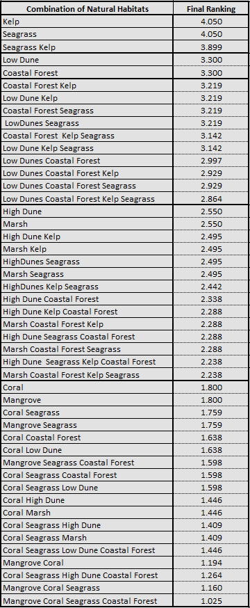
As mentioned in the Natural Habitats section, the model computes the natural habitat exposure ranking for a shoreline segment using equation (115).

This equation is applied to various possible combinations of natural habitats, and the results of this exercise are presented in the table and figure below:

Protection Distance

Ideally this distance is based on empirical study and literature review. Absent of published findings on the distance at which a habitat will protect a coastline from waves, you may estimate this parameter by the following method. View habitat layers in GIS along with the Landmass in your study area. Using a “distance” or “measurement” tool, measure the distance between the shoreline and habitats that you judge to be close enough to have an effect on nearshore coastal processes. It is best to take multiple measurements and develop a sense of an average acceptable distance across your region that can serve as input. Please keep in mind that this distance is reflective of the local bathymetry conditions (a seagrass bed can extend for kilometers seaward in shallow nearshore regions), but also of the quality of the spatial referencing of the input layer.

Wind and Wave data

Wind and Wave data required by the model are included in the InVEST sample data. Below is documentation on how this dataset was created.

To estimate the importance of wind exposure and wind-generated waves, wind statistics measured in the vicinity of the AOI are required. From at least 5 years of data, the model requires the average in each of the 16 equiangular sectors (0deg, 22.5deg, etc.) of the wind speeds in the 90th percentile or greater observed near the segment of interest to compute the Relative Exposure Index (REI; Keddy, 1982). In other words, for computation of the REI, sort wind speed time series in descending order, and take the highest 10% values, and associated direction. Sort this sub-series by direction: all wind speeds that have a direction centered around each of the 16 equiangular sectors are assigned to that sector. Then take the average of the wind speeds in each sector. If there is no record of time series in a particular sector because only weak winds blow from that direction, then average wind speed in that sector is assigned a value of zero (0). Please note that, in the model, wind direction is the direction winds are blowing FROM, and not TOWARDS.

For the computation of wave power from wind and fetch characteristics, the model requires the average of the wind speeds greater than or equal to the 90th percentile observed in each of the 16 equiangular sectors (0deg, 22.5deg, etc.). In other words, for computation of wave power from fetch and wind, sort the time series of observed wind speed by direction: all wind speeds that have a direction centered on each of the 16 equiangular sectors are assigned to that sector. Then, for each sector, take the average of the highest 10% observed values.

If users would like to provide their own wind and wave statistics, instead of relying on WW3 data, you must create a point shapefile with the following columns:

• 16 columns named REI_VX, where X=[0,22,45,67,90,112,135,157,180,202,225,247,270,292,315,337] (e.g., REI_V0). These wind speed values are computed to estimate the REI of each shoreline segment. These values are the average of the highest 10% wind speeds that were allocated to the 16 equiangular sectors centered on the angles listed above.

• 16 columns named REI_PCTX, where X has the same values as listed above. These 16 percent values (which sum to 1 when added together) correspond to the proportion of the highest 10% wind speeds which are centered on the main sector direction X listed above.

• 16 columns named WavP_X, where X has the same values as listed above. These variables are used to estimate wave exposure for sites that are directly exposed to the open ocean. They were computed from WW3 data by first estimating the wave power for all waves in the record, then splitting these wave power values into the 16 fetch sectors defined earlier. For each sector, we then computed WavP by taking the average of the top 10% values (see Section The Model).

• 16 columns named WavPPCTX, where X has the same values as listed above. These variables are used in combination with WavP_X to estimate wave exposure for sites that are directly exposed to the open ocean. They correspond to the proportion of the highest 10% wave power values which are centered on the main sector direction X (see Section The Model).

• 16 columns named V10PCT_X, where X has the same values as listed above. These variables are used to estimate wave power from fetch. They correspond to the average of the highest 10% wind speeds that are centered on the main sector direction X.

Sea level change

Sea level rise is often measured with tide gauges. A good global source of data for tide gauge measurements to be used in the context of sea level rise is the Permanent Service for Sea Level. This site has corrected, and sometimes uncorrected, data on sea-level variation for many locations around the world. To use this in the Coastal Vulnerability Model, you must create a point dataset in GIS representing the location of the tide gauge, and the attribute table must include at least one numeric field of values where larger values indicate a higher level of risk.

References

Arkema, Katie K., Greg Guannel, Gregory Verutes, Spencer A. Wood, Anne Guerry, Mary Ruckelshaus, Peter Kareiva, Martin Lacayo, and Jessica M. Silver. 2013. Coastal Habitats Shield People and Property from Sea-Level Rise and Storms. Nature Climate Change 3 (10): 913–18. https://www.nature.com/articles/nclimate1944.

Bornhold, B.D., 2008, Projected sea level changes for British Columbia in the 21st century, report for the BC Ministry of Environment.

Bush, D.M.; Neal, W.J.; Young, R.S., and Pilkey, O.H. (1999). Utilization of geoindicators for rapid assessment of coastal-hazard risk and mitigation. Oc. and Coast. Manag., 42.

Center for International Earth Science Information Network (CIESIN), Columbia University; and Centro Internacional de Agricultura Tropical (CIAT) (2005). Gridded Population of the World Version 3 (GPWv3). Palisades, NY: Socioeconomic Data and Applications Center (SEDAC), Columbia University.

Cooper J., and McLaughlin S. (1998). Contemporary multidisciplinary approaches to coastal classification and environmental risk analysis. J. Coastal Res. 14(2):512-524

Gornitz, V. (1990). Vulnerability of the east coast, U.S.A. to future sea level rise. JCR, 9.

Gornitz, V. M., Beaty, T.W., and R.C. Daniels (1997). A coastal hazards database for the U.S. West Coast. ORNL/CDIAC-81, NDP-043C: Oak Ridge National Laboratory, Oak Ridge, Tennessee.

Hammar-Klose and Thieler, E.R. (2001). Coastal Vulnerability to Sea-Level Rise: A Preliminary Database for the U.S. Atlantic, Pacific, and Gulf of Mexico Coasts. U.S. Geological Survey, Digital Data Series DDS-68, 1 CD-ROM

Irish, J.L., and Resio, D.T., “A hydrodynamics-based surge scale for hurricanes,” Ocean Eng., Vol. 37(1), 69-81, 2010.

Keddy, P. A. (1982). Quantifying within-lake gradients of wave energy: Interrelationships of wave energy, substrate particle size, and shoreline plants in Axe Lake, Ontario. Aquatic Botany 14, 41-58.

Short AD, Hesp PA (1982). Wave, beach and dune interactions in south eastern Australia. Mar Geol 48:259-284

Tolman, H.L. (2009). User manual and system documentation of WAVEWATCH III version 3.14, Technical Note, U. S. Department of Commerce Nat. Oceanic and Atmosph. Admin., Nat. Weather Service, Nat. Centers for Environmental Pred., Camp Springs, MD.

U.S. Army Corps of Engineers (USACE). 2002. U.S. Army Corps of Engineers Coastal Engineering Manual (CEM) EM 1110-2-1100 Vicksburg, Mississippi.

Wessel, P., and W. H. F. Smith (1996). A Global Self-consistent, Hierarchical, High-resolution Shoreline Database, J. Geophys. Res., 101, #B4, pp. 8741-8743.

World Resources Institute (WRI) (2009). “Value of Coral Reefs & Mangroves in the Caribbean, Economic Valuation Methodology V3.0”.