NDR: Nutrient Delivery Ratio

Summary

The objective of the InVEST nutrient delivery model is to map nutrient sources from watersheds and their transport to the stream. This spatial information can be used to assess the service of nutrient retention by natural vegetation. The retention service is of particular interest for surface water quality issues and can be valued in economic or social terms, such as avoided treatment costs or improved water security through access to clean drinking water.

Introduction

Land use change, and in particular the conversion to agricultural lands, dramatically modifies the natural nutrient cycle. Anthropogenic nutrient sources include point sources, e.g. industrial effluent or water treatment plant discharges, and non-point sources, e.g. fertilizer used in agriculture and residential areas. When it rains or snows, water flows over the landscape carrying pollutants from these surfaces into streams, rivers, lakes, and the ocean. This has consequences for people, directly affecting their health or well-being (Keeler et al., 2012), and for aquatic ecosystems that have a limited capacity to adapt to these nutrient loads.

One way to reduce non-point source pollution is to reduce the amount of anthropogenic inputs (i.e. fertilizer management). When this option fails, ecosystems can provide a purification service by retaining or degrading pollutants before they enter the stream. For instance, vegetation can remove pollutants by storing them in tissue or releasing them back to the environment in another form. Soils can also store and trap some soluble pollutants. Wetlands can slow flow long enough for pollutants to be taken up by vegetation. Riparian vegetation is particularly important in this regard, often serving as a last barrier before pollutants enter a stream.

Land-use planners from government agencies to environmental groups need information regarding the contribution of ecosystems to mitigating water pollution. Specifically, they require spatial information on nutrient export and areas with highest filtration. The nutrient delivery and retention model provides this information for non-point source pollutants. The model was designed for nutrients (nitrogen and phosphorous), but its structure can be used for other contaminants (persistent organics, pathogens etc.) if data are available on the loading rates and filtration rates of the pollutant of interest.

The Model

Overview

The model uses a simple mass balance approach, describing the movement of a mass of nutrient through space. Unlike more sophisticated nutrient models, the model does not represent the details of the nutrient cycle but rather represents the long-term, steady-state flow of nutrients through empirical relationships. Sources of nutrient across the landscape, also called nutrient loads, are determined based on a land use/land cover (LULC) map and associated loading rates. Nutrient loads can then be divided into sediment-bound and dissolved parts, which will be transported through surface and subsurface flow, respectively, stopping when they reach a stream. Note that modeling subsurface flow is optional; the user can choose to model surface flow only. In a second step, delivery factors are computed for each pixel based on the properties of pixels belonging to the same flow path (in particular their slope and retention efficiency of the land use). At the watershed/subwatershed outlet, the nutrient export is computed as the sum of the pixel-level contributions.

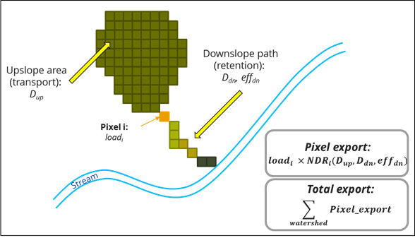
Fig. 5 Conceptual representation of the NDR model. Each pixel i is characterized by its nutrient load, load_i, and its nutrient delivery ratio (NDR), which is a function of the upslope area, and downslope flow path (in particular the retention efficiencies of LULC types on the downslope flow path). Pixel-level export is computed based on these two factors, and the sediment export at the watershed level is the sum of pixel-level nutrient exports.

Nutrient Loads

Loads are the sources of nutrients associated with each pixel of the landscape. Consistent with the export coefficient literature (California Regional Water Quality Control Board Central Coast Region, 2013; Reckhow et al., 1980), load values for each LULC class are derived from empirical measures of nutrient export (e.g. nutrient export running off urban areas, crops, etc.). If information is available on the amount of nutrient applied (e.g. fertilizer, livestock waste, atmospheric deposition), it is possible to use it by estimating the on-pixel nutrient use, and apply this correction factor to obtain the load parameters.

Next, each pixel’s load is modified to account for the local runoff potential. The LULC-based loads defined above are averages for the region, but each pixel’s contribution will depend on the amount of runoff transporting nutrients (Endreny and Wood, 2003; Heathwaite et al., 2005). As a simple approximation, the loads can be modified as follows:

(29)\[modified.load_{x_i}=load_{x_i}\cdot RPI_{x_i}\]

where \(RPI_i\) is the runoff potential index on pixel \(i\), defined as:

(30)\[`RPI_i = RP_i/RP_{av}`\]

where \(RP_i\) is the nutrient runoff proxy for runoff on pixel \(i\) and \(RP_{av}\) is the average \(RP\) over the raster. This approach is similar to that developed by Endreny and Wood (2003). In practice, the raster RP is defined either as a quickflow index (e.g. from the InVEST Seasonal Water Yield model) or as precipitation.

For each pixel, modified loads can be divided into sediment-bound and dissolved nutrient portions. Conceptually, the former represents nutrients that are transported by surface or shallow subsurface runoff, while the latter represent nutrients transported by groundwater. Because phosphorus particles are usually sediment bound and less likely to be transported via subsurface flow, the model uses the subsurface option only for nitrogen (designated by _n) The ratio between these two types of nutrient sources is given by the parameter \(proportion\_subsurface\_n\) which quantifies the ratio of dissolved nutrients over the total amount of nutrients. For a pixel i:

(31)\[load_{surf,i} = (1-proportion\_subsurface_i) \cdot modified.load\_n_i\]

(32)\[load_{subsurf,i} = proportion\_subsurface_i \cdot modified.load\_n_i\]

If no information is available on the partitioning between the two types, the recommended default value of \(proportion\_subsurface\_n\) is 0, meaning that all nutrients are reaching the stream via surface flow. (Note that surface flow can, conceptually, include shallow subsurface flow). However, users should explore the model’s sensitivity to this value to characterize the uncertainty introduced by this assumption.

Nutrient Delivery

Nutrient delivery is based on the concept of nutrient delivery ratio (NDR), an approach inspired by the peer-reviewed concept of sediment delivery ratio (see InVEST SDR User’s Guide chapter and Vigiak et al., 2012). The concept is similar to the risk-based index approaches that are popular for nutrient modeling (Drewry et al., 2011), although it provides quantitative values of nutrient export (e.g. the proportion of the nutrient load that will reach the stream). Two delivery ratios are computed, one for nutrient transported by surface flow, the other for subsurface flow.

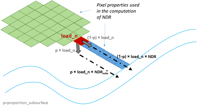
Fig. 6 Conceptual representation of nutrient delivery in the model. If the user chooses to represent subsurface flow, the load on each pixel, load_n, is divided into two parts, and the total nutrient export is the sum of the surface and subsurface contributions.

Surface NDR

The surface NDR is the product of a delivery factor, representing the ability of downstream pixels to transport nutrient without retention, and a topographic index, representing the position on the landscape. For a pixel i:

(33)\[NDR_i = NDR_{0,i}\left(1 + \exp\left(\frac{IC_0-IC_i}{k}\right)\right)^{-1}\]

where \(IC_0\) and \(k\) are calibration parameters, \(IC_i\) is a topographic index, and \(NDR_{0,i}\) is the proportion of nutrient that is not retained by downstream pixels (irrespective of the position of the pixel on the landscape). Below we provide details on the computation of each factor.

\(NDR_{0,i}\) is based on the maximum retention efficiency of the land between a pixel and the stream (downslope path, in Figure 1):

(34)\[NDR_{0,i} = 1 - eff'_i\]

Moving along a flow path, the algorithm computes the additional retention provided by each pixel, taking into account the total distance traveled across each LULC type. Each additional pixel from the same LULC type will contribute a smaller value to the total retention, until the maximum retention efficiency for the given LULC is reached (Figure 2). The total retention is capped by the maximum retention value that LULC types along the flow path can provide, \(eff_{LULC_i}\).

In mathematical terms:

(35)\[\begin{split}eff'_i = \begin{cases} eff_{LULC_i}\cdot(1-s_i) & \mathrm{if\ } down_i \mathrm{\ is\ a\ stream\ pixel}\\ eff'_{down_i}\cdot s_i + eff_{LULC_i}\cdot (1 - s_i) & \mathrm{if\ } eff_{LULC_i} > eff'_{down_i}\\ eff'_{down_i} & otherwise \end{cases}\end{split}\]

Where:

• \(eff'_{down_i}\) is the effective downstream retention on the pixel directly downstream from \(i\),

• \(eff_{LULC_i}\) is the maximum retention efficiency that LULC type \(i\) can reach, and

• \(s_i\) is the step factor defined as:

(36)\[s_i=\exp\left(\frac{-5 \ell_{i_{down}}}{\ell_{LULC_i}}\right)\]

With:

• \(\ell_{i_{down}}\) is the length of the flow path from pixel \(i\) to its downstream neighbor. This is the euclidean distance between the centroids of the two pixels.

• \(\ell_{LULC_i}\) is the LULC retention length (“Critical Length”) of the landcover type on pixel \(i\)

Notes:

Since \(eff'_i\) is dependent on the pixels downstream, calculation proceeds recursively starting at pixels that flow directly into streams before upstream pixels can be calculated.

In equation [6], the factor 5 is based on the assumption that maximum efficiency is reached when 99% of its value is reached (assumption due to the exponential form of the efficiency function, which implies that the maximum value cannot be reached with a finite flow path length).

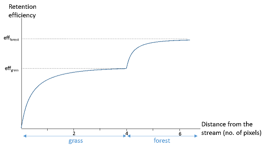
Fig. 7 Illustration of the calculation of the retention efficiency along a simple flow path composed of 4 pixels of grass and 3 pixels of forest. Each additional pixel of the grass LULC contributes to a smaller percentage toward the maximum efficiency provided by grass. The shape of the exponential curves is determined by the maximum efficiency and the retention length.

IC, the index of connectivity, represents the hydrological connectivity, i.e. how likely nutrient on a pixel is likely to reach the stream. In this model, IC is a function of topography only:

(37)\[IC=\log_{10}\left(\frac{D_{up}}{D_{dn}}\right)\]

where

(38)\[D_{up} = \overline{S}\sqrt{A}\]

and

(39)\[D_{dn} = \sum_i \frac{d_i}{S_i}\]

where \(D_{up} = \overline{S}\) is the average slope gradient of the upslope contributing area (m/m), \(A\) is the upslope contributing area (m²); \(d_i\) is the length of the flow path along the ith cell according to the steepest downslope direction (m) (see details in sediment model), and \(S_i\) is the slope gradient of the ith cell, respectively.

Note: The upslope contributing area and downslope flow path are delineated with a Multiple-Flow Direction algorithm. To avoid infinite values for IC, slope values \(S\) are forced to a minimum of 0.005 m/m if they occur to be less than this threshold, based on the DEM (Cavalli et al., 2013).

The value of \(IC_0\) is set to \(IC_0 = \frac{IC_{max}+IC_{min}}{2}\). This imposes that the sigmoid function relating NDR to IC is centered on the median of the IC distribution, hence that the maximum IC value gives \(NDR=NDR_{max}\). \(k\) is set to a default value of 2 (cf. SDR model theory); it is an empirical factor that represents local topography.

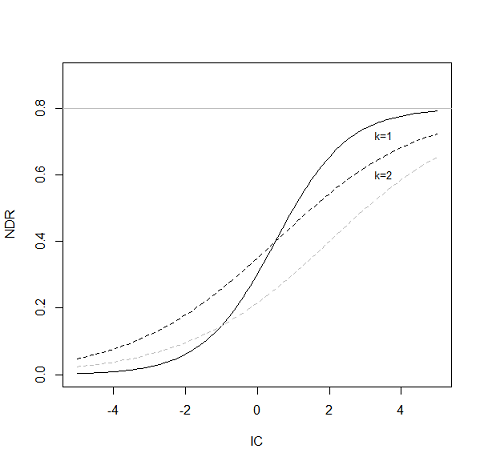
Fig. 8 Relationship between NDR and the connectivity index IC. The maximum value of NDR is set to \(NDR_{0}=0.8\). The effect of the calibration is illustrated by setting \(k=1\) and \(k=2\) (solid and dashed line, respectively), and \(IC_0=0.5\) and \(IC_0=2\) (black and gray dashed lines, respectively).

Subsurface NDR

The expression for the subsurface NDR is a simple exponential decay with distance to stream, plateauing at the value corresponding to the user-defined maximum subsurface nutrient retention:

(40)\[NDR_{subs,i} = 1 - eff_{subs}\left(1-e^\frac{-5\cdot\ell}{\ell_{subs}}\right)\]

where

• \(eff_{subs}\) is the maximum nutrient retention efficiency that can be reached through subsurface flow (i.e. retention due to biochemical degradation in soils),

• \(\ell_{subs}\) is the subsurface flow retention length, i.e. the distance after which it can be assumed that soil retains nutrient at its maximum capacity,

• \(\ell_i\) is the distance from the pixel to the stream.

Nutrient export

Nutrient export from each pixel i is calculated as the product of the load and the NDR:

(41)\[x_{exp_i} = load_{surf,i} \cdot NDR_{surf,i} + load_{subs,i} \cdot NDR_{subs,i}\]

Total nutrient at the outlet of each user-defined watershed is the sum of the contributions from all pixels within that watershed:

(42)\[x_{exp_{tot}} = \sum_i x_{exp_i}\]

Defined Area of Outputs

NDR and several other model outputs are defined in terms of distance to stream (\(d_i\)). Therefore, these outputs are only defined for pixels that drain to a stream on the map (and so are within the streams’ watershed). Pixels that do not drain to any stream will have nodata in these outputs. The affected output files are: d_dn.tif, dist_to_channel.tif, ic_factor.tif, ndr_n.tif, ndr_p.tif, sub_ndr_n.tif, sub_ndr_p.tif, n_export.tif, and p_export.tif.

If you see areas of nodata in these outputs that can’t be explained by missing data in the inputs, it is likely because they are not hydrologically connected to a stream on the map. For an example of what this may look like, see the SDR defined area section.This may happen if your DEM has pits or errors, if the map boundaries do not extend far enough to include streams in that watershed, or if your threshold flow accumulation value is too high to recognize the streams. Check the stream output (stream.tif) and make sure that it aligns as closely as possible with the streams in the real world.

The model’s stream map (stream.tif) is calculated by thresholding the flow accumulation raster (flow_accumulation.tif) by the threshold flow accumulation (TFA) value:

(43)\[\begin{split}stream_{TFA,i} = \left\{\begin{array}{lr} 1, & \text{if } flow\_accum_{i} \geq TFA \\ 0, & \text{otherwise} \\ \end{array}\right\}\end{split}\]

Limitations

The model has a small number of parameters and outputs generally show a high sensitivity to inputs. This implies that errors in the empirical load parameter values will have a large effect on predictions. Similarly, the retention efficiency values are based on empirical studies, and factors affecting these values (like slope or intra-annual variability) are averaged. These values implicitly incorporate information about the dominant nutrient dynamics, influenced by climate and soils. The model also assumes that once nutrient reaches the stream it impacts water quality at the watershed outlet, no in-stream processes are captured. Finally, the effect of grid resolution on the NDR formulation has not been well studied.

Sensitivity analyses are recommended to investigate how the confidence intervals in input parameters affect the study conclusions (Hamel et al., 2015).

Also see the “Biophysical model interpretation” section for further details on model uncertainties.

Options for Valuation

Nutrient export predictions can be used for quantitative valuation of the nutrient retention service. For example, scenario comparison can serve to evaluate the change in purification service between landscapes. The total nutrient load can be used as a reference point, assuming that the landscape has 0 retention. Comparing the current scenario export to the total nutrient load provides a quantitative measure of the retention service of the current landscape.

An important note about assigning a monetary value to any service is that valuation should only be done on model outputs that have been calibrated and validated. Otherwise, it is unknown how well the model is representing the area of interest, which may lead to misrepresentation of the exact value. If the model has not been calibrated, only relative results should be used (such as an increase of 10%) not absolute values (such as 1,523 kg, or 42,900 dollars.)

Data Needs

Raster inputs may have different cell sizes, and they will be resampled to match the cell size of the DEM. Therefore, all model results will have the same cell size as the DEM.

You may choose to run the model with either Nitrogen or Phosphorus or both at the same time. If only one of these is chosen, then all inputs must match. For example, if running Nitrogen, you must provide load_n, eff_n, crit_len_n, Subsurface Critical Length (Nitrogen) and Subsurface Maximum Retention Efficiency (Nitrogen).

• Workspace (required). Folder where model outputs will be written. Make sure that there is ample disk space, and write permissions are correct.

• Suffix (optional). Text string that will be appended to the end of output file names, as “_Suffix”. Use a Suffix to differentiate model runs, for example by providing a short name for each scenario. If a Suffix is not provided, or changed between model runs, the tool will overwrite previous results.

• Digital elevation model (DEM) (required). Raster dataset with an elevation value for each pixel, given in meters. Make sure the DEM is corrected by filling in sinks, and compare the output stream maps with hydrographic maps of the area. To ensure proper flow routing, the DEM should extend beyond the watersheds of interest, rather than being clipped to the watershed edge.

• Land use/land cover (required). Raster of land use/land cover (LULC) for each pixel, where each unique integer represents a different land use/land cover class. All values in this raster MUST have corresponding entries in the Biophysical table.

• Nutrient runoff proxy (required). Raster representing the spatial variability in runoff potential, i.e. the capacity to transport nutrient downstream. This raster can be defined as a quickflow index (e.g. from the InVEST Seasonal Water Yield model) or simply as annual precipitation. The model will normalize this raster (by dividing by its average value) to compute the runoff potential index (RPI, see Eq. (30)). There is not a specific requirement for the units of this input, since it will be normalized by the model before use in calculations.

• Watersheds (required). Shapefile delineating the boundary of the watershed to be modeled. Results will be aggregated within each polygon defined. The column ws_id is required, containing a unique integer value for each polygon.

• Biophysical Table (required). A .csv (Comma Separated Value) table containing model information corresponding to each of the land use classes in the LULC raster. All LULC classes in the LULC raster MUST have corresponding values in this table. Each row is a land use/land cover class and columns must be named and defined as follows:

• lucode (required): Unique integer for each LULC class (e.g., 1 for forest, 3 for grassland, etc.) Every value in the LULC map MUST have a corresponding lucode value in the biophysical table.

• description (optional): Descriptive name of land use/land cover class

• load_n (and/or load_p) (at least one is required): The nutrient loading for each land use class, given as floating point values with units of kilograms per hectare per year. Suffix “_n” stands for nitrogen, and “_p” for phosphorus, and the two compounds can be modeled at the same time or separately.

  Note 1: Loads are the sources of nutrients associated with each LULC class. If you want to represent different levels of fertilizer application, you will need to create separate LULC classes, for example one class called “crops - high fertilizer use” a separate class called “crops - low fertilizer use” etc.

  Note 2: Load values may be expressed either as the amount of nutrient applied (e.g. fertilizer, livestock waste, atmospheric deposition); or as “extensive” measures of contaminants, which are empirical values representing the contribution of a parcel to the nutrient budget (e.g. nutrient export running off urban areas, crops, etc.) In the latter case, the load should be corrected for the nutrient retention from downstream pixels of the same LULC. For example, if the measured (or empirically derived) export value for forest is 3 kg.ha-1.yr-1 and the retention efficiency is 0.8, users should enter 15(kg.ha-1.yr-1) in the n_load column of the biophysical table; the model will calculate the nutrient running off the forest pixel as 15*(1-0.8) = 3 kg.ha-1.yr-1.

• eff_n (and/or eff_p) (at least one is required): The maximum retention efficiency for each LULC class, a floating point value between zero and 1. The nutrient retention capacity for a given vegetation type is expressed as a proportion of the amount of nutrient from upstream. For example, high values (0.6 to 0.8) may be assigned to all natural vegetation types (such as forests, natural pastures, wetlands, or prairie), indicating that 60-80% of nutrient is retained. Like above, suffix “_n” stands for nitrogen, and “_p” for phosphorus, and the two compounds can be modeled at the same time or separately.

• crit_len_n (and/or crit_len_p) (at least one is required): The distance after which it is assumed that a patch of a particular LULC type retains nutrient at its maximum capacity, given in meters. If nutrients travel a distance smaller than the retention length, the retention efficiency will be less than the maximum value eff_x, following an exponential decay (see Nutrient Delivery section).

• proportion_subsurface_n (required if evaluating nitrogen, not required if only evaluating phosphorus): The proportion of dissolved nutrients over the total amount of nutrients, expressed as floating point value (ratio) between 0 and 1. By default, this value should be set to 0, indicating that all nutrients are delivered via surface flow.

An example biophysical table follows, with fields load_p, eff_p and crit_len_p related to the NDR model. Note that these fields are for the case where only phosphorus is being evaluated. This is only to be used as an example, your LULC classes and corresponding values will be different.

description	lucode	usle_c	usle_p	load_p	eff_p	crit_len_p	root_depth	Kc	LULC_veg
Urban and paved roads	1	0.99	1	2.1	0.26	15	0	0.2	0
Grass	3	0.034	1	0.93	0.6	30	2000	0.865	1
General agriculture	5	0.412	1	3.57	0.48	15	1000	1.1	1
Tea	6	0.08135	1	2.47	0.48	15	1850	1.015	1
Coffee	7	0.4393	1	3.81	0.48	15	1600	1.055	1
Forest	8	0.025	1	1.36	0.67	20	3500	1.008	1
Water	9	0	1	0	0.4	15	10	1.05	0
Forest plantation	11	0.121	1	1.4	0.6	20	3500	1.008	1
Unpaved road	18	1	1	0.79	0.26	15	500	0.15	0
Agroforestry	19	0.121	0.6	2.48	0.54	15	3500	1.008	1

• Threshold flow accumulation (required): The number of upstream cells that must flow into a cell before it is considered part of a stream, which is used to classify streams from the DEM. This threshold directly affects the expression of hydrologic connectivity and the nutrient export result: when a flow path reaches the stream, nutrient retention stops and the nutrient exported is assumed to reach the catchment outlet. It is important to choose this value carefully, so modeled streams come as close to reality as possible. See Appendix 1 for more information on choosing this value. Integer value, with no commas or periods - for example “1000”.

• Borselli k parameter (required): Calibration parameter that determines the shape of the relationship between hydrologic connectivity (the degree of connection from patches of land to the stream) and the nutrient delivery ratio (percentage of nutrient that actually reaches the stream; cf. Figure 2). The default value is 2.

• Subsurface Critical Length (Nitrogen or Phosphorus) (required): The distance (traveled subsurface and downslope) after which it is assumed that soil retains nutrient at its maximum capacity, given in meters. If dissolved nutrients travel a distance smaller than Subsurface Critical Length, the retention efficiency will be lower than the Subsurface Maximum Retention Efficiency value defined. Setting this value to a distance smaller than the pixel size will result in the maximum retention efficiency being reached within one pixel only.

• Subsurface Maximum Retention Efficiency (Nitrogen or Phosphorus) (required): The maximum nutrient retention efficiency that can be reached through subsurface flow, a floating point value between 0 and 1. This field characterizes the retention due to biochemical degradation in soils.

Interpreting results

In the file names below, “x” stands for either n (nitrogen) or p (phosphorus), depending on which nutrients were modeled. The resolution of the output rasters will be the same as the resolution of the DEM provided as input.

• Parameter log: Each time the model is run, a text (.txt) file will be created in the Workspace. The file will list the parameter values and output messages for that run and will be named according to the service, date and time. When contacting NatCap about errors in a model run, please include the parameter log.

• [Workspace] folder:

  • watershed_results_ndr_[Suffix].shp: Shapefile which aggregates the nutrient model results per watershed, with “x” in the field names below being n for nitrogen, and p for phosphorus. The .dbf table contains the following information for each watershed:

    • surf_x_ld: Total nutrient loads (sources) in the watershed, i.e. the sum of the nutrient contribution from all surface LULC without filtering by the landscape. [units kg/year]

    • sub_x_ld: Total subsurface nutrient loads in the watershed. [units kg/year]

    • x_exp_tot: Total nutrient export from the watershed.[units kg/year] (Eq. (42))

  • x_export_[Suffix].tif : A pixel level map showing how much load from each pixel eventually reaches the stream. [units: kg/pixel] (Eq. (41))

• [Workspace]\intermediate_outputs folder:

  • crit_len_x: Retention length values, crit_len, found in the biophysical table

  • d_dn: Downslope factor of the index of connectivity (Eq. (39))

  • d_up: Upslope factor of the index of connectivity (Eq. (38))

  • eff_n: Retention efficiencies, eff_x, found in the biophysical table

  • dist_to_channel: Average downstream distance from a pixel to the stream

  • eff_x: Raw per-landscape cover retention efficiency for nutrient x.

  • effective_retention_x: Effective retention provided by the downslope flow path for each pixel (Eq. (35))

  • flow_accumulation: Flow accumulation created from the DEM

  • flow_direction: Flow direction created from the DEM

  • ic_factor: Index of connectivity (Eq. (37))

  • load_x: Loads (for surface transport) per pixel [units: kg/year]

  • modified_load_x: Raw load scaled by the runoff proxy index. [units: kg/year]

  • ndr_x: NDR values (Eq. (33))

  • runoff_proxy_index: Normalized values for the Runoff Proxy input to the model

  • s_accumulation and s_bar: Slope parameters for the IC equation found in the Nutrient Delivery section

  • stream: Stream network created from the DEM, with 0 representing land pixels, and 1 representing stream pixels (Eq. (43)). Compare this layer with a real-world stream map, and adjust the Threshold Flow Accumulation so that this matches real-world streams as closely as possible.

  • sub_crit_len_n: Critical distance value for subsurface transport of nitrogen (constant over the landscape)

  • sub_eff_n: Subsurface retention efficiency for nitrogen (constant over the landscape)

  • sub_effective_retention_n: Subsurface effective retention for nitrogen

  • surface_load_n: Above ground nutrient loads [units: kg/year]

  • sub_load_n: Nitrogen loads for subsurface transport [units: kg/year]

  • sub_ndr_n: Subsurface nitrogen NDR values

  • thresholded_slope: Raster with slope values thresholded for correct calculation of IC.

Biophysical Model Interpretation for Valuation

Some valuation approaches, such as those relying on the changes in water quality for a treatment plant, are very sensitive to the model absolute predictions. Therefore, it is important to consider the uncertainties associated with the use of InVEST as a predictive tool and minimize their effect on the valuation step.

Model parameter uncertainties

Uncertainties in input parameters can be characterized through a literature review (e.g. examining the distribution of values from different studies). One option to assess the impact of parameter uncertainties is to conduct local or global sensitivity analyses, with parameter ranges obtained from the literature (Hamel et al., 2015).

Model structural uncertainties

The InVEST model computes a nutrient mass balance over a watershed, subtracting nutrient losses (conceptually represented by the retention coefficients), from the total nutrient sources. Where relevant, it is possible to distinguish between surface and subsurface flow paths, adding three parameters to the model. In the absence of empirical knowledge, modelers can assume that the surface load and retention parameters represent both transport process. Testing and calibration of the model is encouraged, acknowledging two main challenges:

• Knowledge gaps in nutrient transport: although there is strong evidence of the impact of land use change on nutrient export, modeling of the watershed scale dynamics remains challenging (Breuer et al., 2008; Scanlon et al., 2007). Calibration is therefore difficult and not recommended without in-depth analyses that would provide confidence in model process representation (Hamel et al., 2015)

• Potential contribution from point source pollution: domestic and industrial waste are often part of the nutrient budget and should be accounted for during calibration (for example, by adding point-source nutrient loads to modeled nutrient export, then comparing the sum to observed data).

Comparison to observed data

Despite the above uncertainties, the InVEST model provides a first-order assessment of the processes of nutrient retention and may be compared with observations. Time series of nutrient concentration used for model validation should span over a reasonably long period (preferably at least 10 years) to attenuate the effect of inter-annual variability. Time series should also be relatively complete throughout a year (without significant seasonal data gaps) to ensure comparison with total annual loads. If the observed data is expressed as a time series of nutrient concentration, they need to be converted to annual loads (LOADEST and FLUX32 are two software facilitating this conversion). Additional details on methods and model performance for relative predictions can be found in the study of Hamel and Guswa 2015.

If there are dams on streams in the analysis area, it is possible that they are retaining nutrient, such that it will not arrive at the outlet of the study area. In this case, it may be useful to adjust for this retention when comparing model results with observed data. For an example of how this was done for a study in the northeast U.S., see Griffin et al 2020. The dam retention methodology is described in the paper’s Appendix, and requires knowing the nutrient trapping efficiency of the dam(s).

Appendix: Data sources

Digital Elevation Model

Land Use/Land Cover

Watersheds

Threshold Flow Accumulation

Nutrient Runoff Proxy

Either the quickflow index (e.g. from the InVEST Seasonal Water Yield or other model) or average annual precipitation may be used. Average annual precipitation may be interpolated from existing rain gages, and global data sets from remote sensing models to account for remote areas. When considering rain gage data, make sure that they provide good coverage over the area of interest, especially if there are large changes in elevation that cause precipitation amounts to be heterogeneous within the AOI. Ideally, the gauges will have at least 10 years of continuous data, with no large gaps, around the same time period as the land use/land cover map used.

If field data are not available, you can use coarse annual precipitation data from the freely available global data sets developed by WorldClim (https://www.worldclim.org/) or the Climatic Research Unit (http://www.cru.uea.ac.uk).

Nutrient Load

For all water quality parameters (nutrient load, retention efficiency, and retention length), local literature should be consulted to derive site-specific values. The NatCap nutrient parameter database provides a non-exhaustive list of local references for nutrient loads and retention efficiencies: https://naturalcapitalproject.stanford.edu/sites/g/files/sbiybj9321/f/nutrient_db_0212.xlsx. Parn et al. (2012) and Harmel et al. (2007) provide a good review for agricultural land in temperate climate.

Examples of export coefficients (“extensive” measures, see Data needs) for the US can be found in the EPA PLOAD User’s Manual and in a review by Lin (2004). Note that the examples in the EPA guide are in lbs/ac/yr and must be converted to kg/ha/yr.

Retention Efficiency

This value represents, conceptually, the maximum nutrient retention that can be expected from a given LULC type. Natural vegetation LULC types (such as forests, natural pastures, wetlands, or prairie) are generally assigned high values (>0.8). A review of the local literature and consultation with hydrologists is recommended to select the most relevant values for this parameter. The NatCap nutrient parameter database provides a non-exhaustive list of local references for nutrient loads and retention efficiencies: https://naturalcapitalproject.stanford.edu/sites/g/files/sbiybj9321/f/nutrient_db_0212.xlsx. Parn et al. (2012) provide a useful review for temperate climates. Reviews of riparian buffers efficiency, although a particular case of LULC retention, can also be used as a starting point (Mayer et al., 2007; Zhang et al., 2009).

Retention Length: crit_len_n and crit_len_p

This value represents the typical distance necessary to reach the maximum retention efficiency. It was introduced in the model to remove any sensitivity to the resolution of the LULC raster. The literature on riparian buffer removal efficiency suggests that retention lengths range from 10 to 300 m (Mayer et al., 2007; Zhang et al., 2009). In the absence of local data for land uses that are not forest or grass, you can simply set the retention length constant, equal to the pixel size: this will result in the maximum retention efficiency being reached within a distance of one pixel only. Another option is to treat the retention length as a calibration parameter. In the absence of any other information, start with a value at the mid-point of the range given above (that is, 150m), then vary that value up and down during calibration to find a good fit.

Subsurface Parameters: proportion_subsurface_n, eff_sub, crit_len_sub

These values are used for advanced analyses and should be selected in consultation with hydrologists. Parn et al. (2012) provide average values for the partitioning of N loads between leaching and surface runoff. From Mayer et al. (2007), a global average of 200m for the retention length, and 80% for retention efficiency can be assumed for vegetated buffers.

References

Breuer, L., Vaché, K.B., Julich, S., Frede, H.-G., 2008. Current concepts in nitrogen dynamics for mesoscale catchments. Hydrol. Sci. J. 53, 1059–1074.

California Regional Water Quality Control Board Central Coast Region, 2013. Total Maximum Daily Loads for Nitrogen Compounds and Orthophosphate for the Lower Salinas River and Reclamation Canal Basin , and the Moro Cojo Slough Subwatershed , Monterey County, CA. Appendix F. Available at: https://www.waterboards.ca.gov/centralcoast/water_issues/programs/tmdl/docs/salinas/nutrients/index.html

Endreny, T.A., Wood, E.F., 2003. Watershed weighting of export coefficients to map critical phosphorous loading areas. J. Am. Water Resour. Assoc. 08544, 165–181.

Robert Griffin, Adrian Vogl, Stacie Wolny, Stefanie Covino, Eivy Monroy, Heidi Ricci, Richard Sharp, Courtney Schmidt, Emi Uchida, 2020. “Including Additional Pollutants into an Integrated Assessment Model for Estimating Nonmarket Benefits from Water Quality,” Land Economics, University of Wisconsin Press, vol. 96(4), pages 457-477. DOI: 10.3368/wple.96.4.457

Hamel, P., Chaplin-Kramer, R., Sim, S., Mueller, C., 2015. A new approach to modeling the sediment retention service (InVEST 3.0): Case study of the Cape Fear catchment, North Carolina, USA. Sci. Total Environ. 166–177.

Hamel, P., Guswa A.J. 2015. Uncertainty Analysis of the InVEST 3.0 Nutrient Model: Case Study of the Cape Fear Catchment, NC. Hydrology and Earth System Sciences Discussion 11:11001-11036. http://dx.doi.org/10.5194/hessd-11-11001-2014

Harmel, D., Potter, S., Casebolt, P., Reckhow, K., 2007. Compilation of measured nutrient load data for agricultural land uses in the United States 76502, 1163–1178.

Heathwaite, A.L., Quinn, P.F., Hewett, C.J.M., 2005. Modelling and managing critical source areas of diffuse pollution from agricultural land using flow connectivity simulation. J. Hydrol. 304, 446–461.

Keeler, B.L., Polasky, S., Brauman, K.A., Johnson, K.A., Finlay, J.C., Neill, A.O., 2012. Linking water quality and well-being for improved assessment and valuation of ecosystem services 109, 18629–18624.

Lin, J.., 2004. Review of published export coefficient and event mean concentration (EMC) data, WRAP Technical Notes Collection (ERDC TN-WRAP-04-3). Vicksburg, MS.

Mayer, P.M., Reynolds, S.K., Mccutchen, M.D., Canfield, T.J., 2007. Meta-Analysis of Nitrogen Removal in Riparian Buffers 1172–1180.

Pärn, J., Pinay, G., Mander, Ü., 2012. Indicators of nutrients transport from agricultural catchments under temperate climate: A review. Ecol. Indic. 22, 4–15.

Reckhow, K.H., Beaulac, M.N., Simpson, J.T., 1980. Modeling Phosphorus loading and lake response under uncertainty: A manual and compilation of export coefficients. EPA 440/5-80-011. US-EPA, Washington, DC.

Scanlon, B.R., Jolly, I., Sophocleous, M., Zhang, L., 2007. Global impacts of conversions from natural to agricultural ecosystems on water resources: Quantity versus quality. Water Resour. Res. 43.

Tarboton, D., 1997. A new method for the determination of flow directions and upslope areas in grid digital elevation models. Water Resour. Res. 33, 309–319.

Vigiak, O., Borselli, L., Newham, L.T.H., Mcinnes, J., Roberts, A.M., 2012. Comparison of conceptual landscape metrics to define hillslope-scale sediment delivery ratio. Geomorphology 138, 74–88.

Zhang, X., Liu, X., Zhang, M., Dahlgren, R. a, Eitzel, M., 2009. A review of vegetated buffers and a meta-analysis of their mitigation efficacy in reducing nonpoint source pollution. J. Environ. Qual. 39, 76–84.