Annual Water Yield
Summary
Hydropower accounts for twenty percent of worldwide energy production, most of which is generated by reservoir systems. InVEST estimates the annual average quantity and value of hydropower produced by reservoirs, and identifies how much water yield or value each part of the landscape contributes annually to hydropower production. The model has three components: water yield, water consumption, and hydropower valuation. The biophysical models do not consider surface – ground water interactions or the temporal dimension of water supply. The valuation model assumes that energy pricing is static over time.
Introduction
The provision of fresh water is an ecosystem service that contributes to the welfare of society in many ways, including through the production of hydropower, the most widely used form of renewable energy in the world. Most hydropower production comes from watershed-fed reservoir systems that generally deliver energy consistently and predictably. The systems are designed to account for annual variability in water volume, given the likely levels for a given watershed, but are vulnerable to extreme variation caused by land use and land cover (LULC) changes. LULC changes can alter hydrologic cycles, affecting patterns of evapotranspiration, infiltration and water retention, and changing the timing and volume of water that is available for hydropower production (World Commission on Dams 2000; Ennaanay 2006).
Changes in the landscape that affect annual average water yield upstream of hydropower facilities can increase or decrease hydropower production capacity. Maps of where water yield used for hydropower is produced can help avoid unintended impacts on hydropower production or help direct land use decisions that wish to maintain power production, while balancing other uses such as conservation or agriculture. Such maps can also be used to inform investments in restoration or management that downstream stakeholders, such as hydropower companies, make in hopes of improving or maintaining water yield for this important ecosystem service. In large watersheds with multiple reservoirs for hydropower production, areas upstream of power plants that sell to a higher value market will have a higher value for this service. Maps of how much value each parcel contributes to hydropower production can help managers avoid developments in the highest hydropower value areas, understand how much value will be lost or gained as a consequence of different management options, or identify which hydropower producers have the largest stake in maintaining water yield across a landscape.
The Model
The InVEST Water Yield model estimates the relative contributions of water from different parts of a landscape, offering insight into how changes in land use patterns affect annual surface water yield and hydropower production.
Modeling the connections between landscape changes and hydrologic processes is not simple. Sophisticated models of these connections and associated processes (such as the WEAP model) are resource and data intensive and require substantial expertise. To accommodate more contexts, for which data are readily available, InVEST maps and models the annual average water yield from a landscape used for hydropower production, rather than directly addressing the effect of LULC changes on hydropower, as this process is closely linked to variation in water inflow on a daily to monthly timescale. Instead, InVEST calculates the relative contribution of each land parcel to annual average hydropower production and the value of this contribution in terms of energy production. The net present value of hydropower production over the life of the reservoir also can be calculated by summing discounted annual revenues.
How it Works
The model runs on a gridded map. It estimates the quantity and value of water used for hydropower production from each subwatershed in the area of interest. It has three components, which run sequentially. First, it determines the amount of water running off each pixel as the precipitation minus the fraction of the water that undergoes evapotranspiration. The model does not differentiate between surface, subsurface and baseflow, but assumes that all water yield from a pixel reaches the point of interest via one of these pathways. This model then sums and averages water yield to the subwatershed level. The pixel-scale calculations allow us to represent the heterogeneity of key driving factors in water yield such as soil type, precipitation, vegetation type, etc. However, the theory we are using as the foundation of this set of models was developed at the subwatershed to watershed scale. We are only confident in the interpretation of these models at the subwatershed scale, so all outputs are summed and/or averaged to the subwatershed scale. We do continue to provide pixel-scale representations of some outputs for calibration and model-checking purposes only. These pixel-scale maps are not to be interpreted for understanding of hydrological processes or to inform decision making of any kind.
Second, beyond annual average runoff, it calculates the proportion of surface water that is available for hydropower production by subtracting the surface water that is consumed for other uses. Third, it estimates the energy produced by the water reaching the hydropower reservoir and the value of this energy over the reservoir’s lifetime.
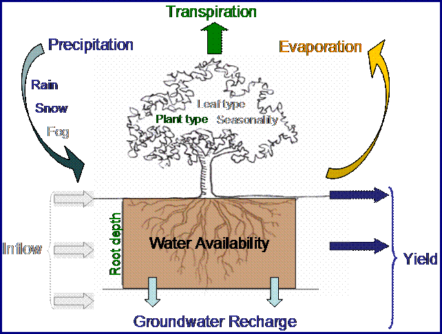
Figure 1. Conceptual diagram of the simplified water balance method used in the annual water yield model. Aspects of the water balance that are in color are included in the model, those that are in grey are not.
Water Yield Model
The water yield model is based on the Budyko curve and annual average precipitation. We determine annual water yield \(Y(x)\) for each pixel on the landscape \(x\) as follows:
where \(AET(x)\) is the annual actual evapotranspiration for pixel \(x\) and \(P(x)\) is the annual precipitation on pixel \(x\).
For vegetated land use/land cover (LULC) types, the evapotranspiration portion of the water balance, \(\frac{AET(x)}{P(x)}\) , is based on an expression of the Budyko curve proposed by Fu (1981) and Zhang et al. (2004):
where \(PET(x)\) is the potential evapotranspiration and \(\omega(x)\) is a non-physical parameter that characterizes the natural climatic-soil properties, both detailed below.
Potential evapotranspiration \(PET(x)\) is defined as:
where, \(ET_0(x)\) is the reference evapotranspiration from pixel \(x\) and \(K_c(\ell_x)\) is the plant (vegetation) evapotranspiration coefficient associated with the LULC \(\ell_x\) on pixel \(x\). \(ET_0(x)\) reflects local climatic conditions, based on the evapotranspiration of a reference vegetation such as grass or alfalfa grown at that location. \(K_c(\ell_x)\) is largely determined by the vegetative characteristics of the land use/land cover found on that pixel (Allen et al. 1998). \(K_c\) adjusts the \(ET_0\) values to the crop or vegetation type in each pixel of the land use/land cover map.
\(\omega(x)\) is an empirical parameter that can be expressed as linear function of \(\frac{AWC*N}{P}\), where N is the number of rain events per year, and AWC is the volumetric plant available water content (see Appendix 1 for additional details). While further research is being conducted to determine the function that best describe global data, we use the expression proposed by Donohue et al. (2012) in the InVEST model, and thus define:
where:
\(AWC(x)\) is the volumetric (mm) plant available water content. The soil texture and effective rooting depth define \(AWC(x)\), which establishes the amount of water that can be held and released in the soil for use by a plant. It is estimated as the product of the plant available water capacity (PAWC) and the minimum of root restricting layer depth and vegetation rooting depth:
\[AWC(x)= Min(Rest.layer.depth, root.depth)\cdot PAWC\]Root restricting layer depth is the soil depth at which root penetration is inhibited because of physical or chemical characteristics. Vegetation rooting depth is often given as the depth at which 95% of a vegetation type’s root biomass occurs. PAWC is the plant available water capacity, i.e. the difference between field capacity and wilting point.
\(Z\) is an empirical constant, sometimes referred to as “seasonality factor”, which captures the local precipitation pattern and additional hydrogeological characteristics. It is positively correlated with N, the number of rain events per year. The 1.25 term is the minimum value of \(\omega(x)\), which can be seen as a value for bare soil (when root depth is 0), as explained by Donohue et al. (2012). Following the literature (Yang et al., 2008; Donohue et al. 2012), values of \(\omega(x)\) are capped to a value of 5.
For other LULC types (open water, urban, wetland), actual evapotranspiration is directly computed from reference evapotranspiration \(ET_0(x)\) and has an upper limit defined by precipitation:
where \(ET_0(x)\) is reference evapotranspiration, and \(K_c(\ell_x)\) is the evaporation factor for each LULC.
The water yield model generates and outputs the total and average water yield at the subwatershed level.
Realized Supply
The Realized Supply option of the model (called Water Scarcity in the tool interface) calculates the water inflow to a reservoir based on calculated water yield and water consumptive use in the watershed(s) of interest. The user inputs how much water is consumed by each land use/land cover type in a table format. Examples of consumptive use include municipal or industrial withdrawals that are not returned to the stream upstream of the outlet. This option may also be used to represent inter-basin transfers out of the study watershed.
For example, in an urban area, consumptive use can be calculated as the product of population density and per capita consumptive use. These land use-based values only relate to the consumptive portion of demand; some water use is non-consumptive such as water used for industrial processes or waste water that is returned to the stream after use, upstream of the outlet. Consumptive use estimates should therefore take into account any return flows to the stream above the watershed outlet:
where, \(C\) = the consumptive use (\(m^3/yr/pixel\)), \(W\) = withdrawals (\(m^3/yr\)), \(R\) = return flows (\(m^3/yr\)), and \(n\) = number of pixels in a given land cover.
For simplicity, each pixel in the watershed is either a “contributing” pixel, which contributes to hydropower production, or a “use” pixel, which uses water for other consumptive uses. This assumption implies that land use associated with consumptive uses will not contribute any yield for downstream use. The amount of water that actually reaches the reservoir for dam \(d\) (called realized supply) is defined as the difference between total water yield from the watershed and total consumptive use in the watershed:
where \(V_{in}\) is the realized supply (volume inflow to a reservoir), \(u_d\) is the total volume of water consumed in the watershed upstream of dam \(d\) and \(Y\) is the total water yield from the watershed upstream of dam \(d\).
Note that only anthropogenic uses are considered here, since evapotranspiration (including consumptive use of water by croplands) are accounted for by the \(K_c\) parameter in the water yield model. Users should be aware that the model assumes that all water available for evapotranspiration comes from within the watershed (as rainfall). This assumption holds true in cases where agriculture is either rain-fed, or the source of irrigation water is within the study watershed (not sourced from inter-basin transfer or a disconnected deeper aquifer). See the Limitations section for more information on applying the model in watersheds with irrigated agriculture.
If observed data is available for actual annual inflow rates to the reservoir for dam \(d\), they can be compared to \(V_{in}\).
Hydropower Production and Valuation
The Valuation option of the model estimates both the amount of energy produced given the estimated realized supply of water for hydropower production and the value of that energy. A present value monetary estimate is given for the entire remaining lifetime of the reservoir. Net present value can be calculated if hydropower production cost data are available. The energy produced and the revenue is then redistributed over the landscape based on the proportional contribution of each subwatershed to energy production. Final output maps show how much energy production and hydropower value can be attributed to each subwatershed’s water yield over the lifetime of the reservoir.
An important note about assigning a monetary value to any service is that valuation should only be done on model outputs that have been calibrated and validated. Otherwise, it is unknown how well the model is representing the area of interest, which may lead to misrepresentation of the exact value. If the model has not been calibrated, only relative results should be used (such as an increase of 10%) not absolute values (such as 1,523 cubic meters, or 42,900 dollars.)
At dam \(d\), power is calculated using the following equation:
where \(p_d\) is power in watts, \(\rho\) is the water density (1000 Kg/m3), \(q_d\) is the flow rate (m3/s), \(g\) is the gravity constant (9.81 m/s2), and \(h_d\) is the water height behind the dam at the turbine (m). In this model, we assume that the total annual inflow water volume is released equally and continuously over the course of each year.
The power production equation is connected to the water yield model by converting the annual inflow volume adjusted for consumption (\(V_{in}\)) to a per second rate. Since electric energy is normally measured in kilowatt-hours, the power \(p_d\) is multiplied by the number of hours in a year. All hydropower reservoirs are built to produce a maximum amount of electricity. This is called the energy production rating, and represents how much energy could be produced if the turbines are 100% efficient and all water that enters the reservoir is used for power production. In the real world, turbines have inefficiencies and water in the reservoir may be extracted for other uses like irrigation, retained in the reservoir for other uses like recreation, or released from the reservoir for non-power production uses like maintaining environmental flows downstream. To account for these inefficiencies and the flow rate and power unit adjustments, annual average energy production \(\varepsilon_d\) at dam \(d\) is calculated as follows:
where \(\varepsilon_d\) is hydropower energy production (KWH), \(\beta\) is the turbine efficiency coefficient (%), \(\gamma_d\) is the percent of inflow water volume to the reservoir at dam \(d\) that will be used to generate energy.
To convert \(\varepsilon_d\), the annual energy generated by dam \(d\), into a net present value (NPV) of energy produced (point of use value) we use the following,
where \(TC_d\) is the total annual operating costs for dam \(d\), \(p_e\) is the market value of electricity (per kilowatt hour) provided by the hydropower plant at dam \(d\), \(T_d\) indicates the number of years present landscape conditions are expected to persist or the expected remaining lifetime of the station at dam \(d\) (set \(T\) to the smallest value if the two time values differ), and \(r\) is the market discount rate. The form of the equation above assumes that \(TC_d\), \(p_e\), and \(\varepsilon_d\), are constant over time.
Energy production over the lifetime of dam \(d\) is attributed to each subwatershed as follows:
where the first term in parentheses represents the electricity production over the lifetime of dam \(d\). The second term represents the proportion of water volume used for hydropower production that comes from subwatershed \(x\) relative to the total water volume for the whole watershed. The value of each subwatershed for hydropower production over the lifetime of dam \(d\) is calculated similarly:
Limitations and Simplifications
The model has a number of limitations. First, it is not intended for devising detailed water plans, but rather for evaluating how and where changes in a watershed may affect hydropower production for reservoir systems. It is based on annual averages, which neglect extremes and do not consider the temporal dimensions of water supply and hydropower production.
Second, the model does not consider the spatial distribution of land use/land cover. The empirical model used for the water balance (based on the Budyko theory) has been tested at larger scales than the pixel dimensions used in InVEST (Hamel & Guswa, in review). Complex land use patterns or underlying geology, which may induce complex water balances, may not be well captured by the model.
Third, the model does not consider sub-annual patterns of water delivery timing. Water yield is a provisioning function, but hydropower benefits are also affected by flow regulation. The timing of peak flows and delivery of minimum operational flows throughout the year determines the rate of hydropower production and annual revenue. Changes in landscape scenarios are likely to affect the timing of flows as much as the annual water yield, and are of particular concern when considering drivers such as climate change. Modeling the temporal patterns of overland flow requires detailed data that are not appropriate for our approach. Still, this model provides a useful initial assessment of how landscape scenarios may affect the annual delivery of water to hydropower production.
Fourth, the model greatly simplifies consumptive demand. For each LULC, a single variable (\(\gamma_d\)) is used to represent multiple aspects of water resource allocation, which may misrepresent the complex distribution of water among uses and over time. In reality, water demand may differ greatly between parcels of the same LULC class. Much of the water demand may also come from large point source intakes, which are not represented by an LULC class at all. The model simplifies water demand by distributing it over the landscape. For example, the water demand may be large for an urban area, and the model represents this demand by distributing it over the urban LULC class. The actual water supply intake, however, is likely further upstream in a rural location. Spatial disparity in actual and modeled demand points may cause an incorrect representation in the realized supply output grid. The distribution of consumption is also simplified in the reallocation of energy production and hydropower value since it is assumed that water consumed along flow paths is drawn equally from every pixel upstream. As a result, water scarcity, energy production patterns, and hydropower values may be incorrectly estimated.
Fifth, water transfers for irrigation, either between subbasins or between seasons, are not well captured by the model. When applying the empirical approach to cropland, irrigation patterns should be considered, which typically fall into one of the following cases:
If there is no irrigation other than direct rain, it can be assumed that croplands respond to climate forcing in a similar way to natural vegetation (i.e. the theory behind the eco-hydrological model used in the InVEST model, linking plant available water and climate forcing, applies, cf. Donohue et al. 2012)
If small reservoirs store water during the wet season to irrigate crops during the dry season, the AET should equal PET during the irrigation season. However, the model predicts AET<PET due to limited water retention in undisturbed catchments (where there is no other reservoir except soil storage). This likely results in the underestimation of evapotranspiration, and therefore the overestimation of yields. To avoid this issue, you can use the alternative equation for AET (equation 2), which sets AET directly as a function of ETo. (In that case, remember that AET is capped by P to avoid predicting negative water yields, which may result in an overestimation of yields).
If the study area contains croplands that are irrigated with water from outside the catchment (either through inter-basin transfer or pumping from a disconnected groundwater source), then AET also equals PET during the irrigation season. Because the model assumes that evapotranspiration is sourced from rainfall, the water yield output is likely overestimated. This situation can also be represented by using the alternative equation for AET (equation 2). Assuming that crops are being irrigated efficiently (i.e. the total volume of imported water is equal to the water deficit, or PET – P, for crop pixels), then the known volume of water irrigated may be added to the modeled water yield to give a better picture of actual yield.
Because seasonality can play a significant role in irrigation water use, use caution when applying the annual model in catchments with large irrigated fields. For options that are not covered above or where complex water transfers may substantially affect the water balance, users are encouraged to use alternative models that will better represent the spatial and temporal water transfers. In particular, great caution should be used when calibrating the model without good data on the different water balance components within your study area (i.e. rainfall, streamflow, irrigation rates and timing).
Finally, the model assumes that hydropower production and pricing remain constant over time. It does not account for seasonal variation in energy production or fluctuations in energy pricing, which may affect the value of hydropower. Even if sub-annual production or energy prices change, however, the relative value between parcels of land in the same drainage area should be accurate.
Data Needs
Raster inputs may have different cell sizes, and they will be resampled to match the cell size of the land use/land cover raster. Therefore, all model results will have the same cell size as the land use/land cover raster.
Workspace (required). Folder where model outputs will be written. Make sure that there is ample disk space, and write permissions are correct.
Suffix (optional). Text string that will be appended to the end of output file names, as “_Suffix”. Use a Suffix to differentiate model runs, for example by providing a short name for each scenario. If a Suffix is not provided, or changed between model runs, the tool will overwrite previous results.
Precipitation (required). A GIS raster dataset with a non-zero value for average annual precipitation for each cell. [units: millimeters]
Average Annual Reference Evapotranspiration (required). A GIS raster dataset, with an annual average evapotranspiration value for each cell. Reference evapotranspiration is the potential loss of water from soil by both evaporation from the soil and transpiration by healthy alfalfa (or grass) if sufficient water is available. [units: millimeters]
Root restricting layer depth (required). A GIS raster dataset with an average root restricting layer depth value for each cell. Root restricting layer depth is the soil depth at which root penetration is strongly inhibited because of physical or chemical characteristics. [units: millimeters]
Plant Available Water Content (required). A GIS raster dataset with a plant available water content value for each cell. Plant Available Water Content fraction (PAWC) is the fraction of water that can be stored in the soil profile that is available for plants’ use. [fraction from 0 to 1]
Land use/land cover (required). A GIS raster dataset, with an integer LULC code for each cell. These LULC codes must match lucode values in the Biophysical table.
Watersheds (required). A shapefile, with one polygon per watershed. This is a layer of watersheds such that each watershed contributes to a point of interest where hydropower production will be analyzed. An integer field named ws_id is required, with a unique integer value for each watershed.
Subwatersheds (required). A shapefile, with one polygon per subwatershed within the main watersheds specified in the Watersheds shapefile. An integer field named subws_id is required, with a unique integer value for each subwatershed.
Biophysical Table (required). A .csv (Comma Separated Value) table containing model information corresponding to each of the land use classes in the LULC raster. All LULC classes in the LULC raster MUST have corresponding values in this table. Each row is a land use/land cover class and columns must be named and defined as follows:
lucode (required): Unique integer for each LULC class (e.g., 1 for forest, 3 for grassland, etc.) Every value in the LULC map MUST have a corresponding lucode value in the biophysical table.
LULC_desc (optional): Descriptive name of land use/land cover class
LULC_veg (required): Specifies which AET equation to use (Eq. 1 or 2). Values must be 1 for vegetated land use except wetlands, and 0 for all other land uses, including wetlands, urban, water bodies, etc.
root_depth (required): The maximum root depth for vegetated land use classes, given in integer millimeters. This is often given as the depth at which 95% of a vegetation type’s root biomass occurs. For land uses where the generic Budyko curve is not used (i.e. where evapotranspiration is calculated from Eq. 2), rooting depth is not needed. In these cases, the rooting depth field is ignored, and may be set as a value such as -1 to indicate the field is not used.
Kc (required): Plant evapotranspiration coefficient for each LULC class, used to calculate potential evapotranspiration by using plant physiological characteristics to modify the reference evapotranspiration, which is based on alfalfa. The evapotranspiration coefficient is a decimal in the range of 0 to 1.5 (some crops evapotranspire more than alfalfa in some very wet tropical regions and where water is always available).
Z parameter (required). Floating point value on the order of 1 to 30 corresponding to the seasonal distribution of precipitation (see the Appendix for more information).
Demand Table (required if calculating Water Scarcity or Valuation). A table of LULC classes, with consumptive water use for each landuse/landcover type. Consumptive water use is that part of water used that is incorporated into products or crops, consumed by humans or livestock, or otherwise removed from the watershed water balance. Each row is a land use/land cover class, and columns must be named and defined as follows:
lucode (required): Unique integer for each LULC class (e.g., 1 for forest, 3 for grassland, etc.), must match the LULC raster above.
demand (required): The estimated average consumptive water use for each landuse/landcover type. Demand must be given in cubic meters per year per pixel in the land use/land cover map. Note that accounting for pixel area is important since larger pixels will consume more water for the same land cover type.
Hydropower valuation table (required if doing Valuation). A table of hydropower stations (which are the outlets of the input Watersheds) with associated model values. Each row is a hydropower station, and columns must be named and defined as follows:
ws_id (required): Unique integer value for each hydropower station, which must correspond to values in the Watersheds layer.
station_desc (optional): Name of hydropower station
efficiency (required): Turbine efficiency, obtained from the hydropower plant manager. Floating point values (generally 0.7 to 0.9).
fraction (required): The fraction of inflow water volume that is used to generate energy, obtained from the hydropower plant manager. Managers can release water without generating electricity to satisfy irrigation, drinking water or environmental demands. Floating point value.
height (required): The head, measured as the average annual effective height of water behind each dam at the turbine intake. Floating point value in meters.
kw_price (required): The price of one kilowatt-hour of power produced by the station, in any currency (but must match the currency used for cost.) Floating point value.
cost (required): Annual cost of running the hydropower station (maintenance and operations costs), in any currency (but must match the currency used for kw_price.) Floating point value.
time_span (required): Either the expected lifespan of the hydropower station or the period of time of the land use scenario of interest, expressed as number of years. Used in net present value calculations. Integer value.
discount (required): The discount rate over the time span, used in net present value calculations. Percentage - for example, if the discount rate is 5%, enter the value 5.
Interpreting Results
The resolution of the output rasters will be the same as the resolution of the Land use/land cover raster provided as input.
Parameter log: Each time the model is run, a text (.txt) file will be created in the Workspace. The file will list the parameter values and output messages for that run and will be named according to the service, the date and time. When contacting NatCap about errors in a model run, please include the parameter log.
Outputs in the per_pixel folder can be useful for intermediate calculations but should NOT be interpreted at the pixel level, as model assumptions are based on processes understood at the subwatershed scale.
output\per_pixel\fractp_[Suffix].tif (fraction): Estimated actual evapotranspiration fraction of precipitation per pixel (Actual Evapotranspiration / Precipitation). It is the mean fraction of precipitation that actually evapotranspires at the pixel level.
output\per_pixel\aet_[Suffix].tif (mm): Estimated actual evapotranspiration per pixel.
output\per_pixel\wyield_[Suffix].tif (mm): Estimated water yield per pixel.
output\subwatershed_results_wyield_[Suffix].shp and output\subwatershed_results_wyield_[Suffix].csv: Shapefile and table containing biophysical output values per subwatershed, with the following attributes:
precip_mn (mm): Mean precipitation per pixel in the subwatershed.
PET_mn (mm): Mean potential evapotranspiration per pixel in the subwatershed.
AET_mn (mm): Mean actual evapotranspiration per pixel in the subwatershed.
wyield_mn (mm): Mean water yield per pixel in the subwatershed.
wyield_vol (m3): Volume of water yield in the subwatershed.
output\watershed_results_wyield_[Suffix].shp and output\watershed_results_wyield_[Suffix].csv: Shapefile and table containing output values per watershed, with the following attributes:
precip_mn (mm): Mean precipitation per pixel in the watershed.
PET_mn (mm): Mean potential evapotranspiration per pixel in the watershed.
AET_mn (mm): Mean actual evapotranspiration per pixel in the watershed.
wyield_mn (mm): Mean water yield per pixel in the watershed.
wyield_vol (m3): Volume of water yield in the watershed.
If the Water Scarcity option is run, the following attributes will also be included for watersheds and subwatersheds:
consum_vol (m3): Total water consumption for each watershed.
consum_mn (m3/ha): Mean water consumptive volume per pixel per watershed.
rsupply_vl (m3): Total realized water supply (water yield – consumption) volume for each watershed.
rsupply_mn (m3/ha): Mean realized water supply (water yield – consumption) volume per pixel per watershed.
If the Valuation option is run, the following attributes will also be included for watersheds, but not for subwatersheds:
hp_energy (kw/timespan): The amount of ecosystem service in energy production terms. This shows the amount of energy produced by the hydropower station over the specified timespan that can be attributed to each watershed based on its water yield contribution.
hp_val (currency/timespan): The amount of ecosystem service in economic terms. This shows the value of the landscape per watershed according to its ability to yield water for hydropower production over the specified timespan.
intermediate: This directory contains data that represent intermediate steps in calculations of the final data in the output folder. It also contains subdirectories that store metadata used internally to enable avoided re-computation.
The application of these results depends entirely on the objective of the modeling effort. Users may be interested in all of these results or a select one or two. If valuation information is not available or of interest, you may choose to simply run the water yield model and compare biophysical results.
The first several model results provide insight into how water is distributed throughout the landscape. aet_mn describes the actual evapotranspiration depth of the hydrologic cycle, showing how much water (precipitation) is lost annually to evapotranspiration across the watershed or subwatershed.
The wyield_vol field contains the estimated annual average water volume that is ‘yielded’ from each subwatershed within the watershed of interest. This value can be used to determine which subwatersheds are most important to total annual water yield – although at this step the user still will not know how much of that water is benefiting downstream users of any type. The consumptive use (consum_vol) field then shows how much water is used for consumptive activities (such as drinking, bottling, etc.) each year across the landscape per watershed. The realized supply (rsupply_vl) field contains the difference between cumulative water yield and cumulative consumptive use. This value demonstrates where the water supply for hydropower production is abundant and where it is most scarce. Remember that the consumptive use value may not truly represent where water is taken, only where it is demanded. This may cause some misrepresentation of the scarcity in certain locations, but this value offers a general sense of the water balance and whether there is a lack of or abundance of water in the watershed of interest.
The hp_energy and hp_val values are the most relevant model outputs for prioritizing the landscape for investments that wish to maintain water yield for hydropower production. The hp_val field contains the most information for this purpose as it represents the revenue attributable to each watershed over the expected lifetime of the hydropower station, or the number of years that the user has chosen to model. This value accounts for the fact that different hydropower stations within a large river basin may have different customers who pay different rates for energy production. If this is the case, this result will show which watersheds contribute the highest value water for energy production. If energy values do not vary much across the landscape, the hp_energy outputs can be just as useful in planning and prioritization. Comparing any of these values between landuse scenarios allows you to understand how the role of the landscape may change under different management plans.
Appendix 1: Data Sources
Precipitation
Reference Evapotranspiration
Kc
Land Use/Land Cover
Watersheds/Subwatersheds
Root restricting layer depth
Root restricting layer depth is the soil depth at which root penetration is strongly inhibited because of physical or chemical characteristics. Root restricting layer depth may be obtained from some soil maps. If root restricting layer depth or rootable depth by soil type is not available, soil depth can be used as a proxy. If several soil horizons are detailed, the root restricting layer depth is the sum of the depths of non-restrictive soil horizons.
Global soil data are available from the Soil and Terrain Database (SOTER) Programme (https://data.isric.org:443/geonetwork/srv/eng/catalog.search). They provide some area-specific soil databases, as well as SoilGrids globally. Type “depth” into their Search engine to see a list of layers. For SoilGrids, Depth to bedrock (R horizon) can be used.
The FAO also provides global soil data in their Harmonized World Soil Database: https://webarchive.iiasa.ac.at/Research/LUC/External-World-soil-database/HTML/, but it is rather coarse.
In the United States free soil data is available from the U.S. Department of Agriculture’s NRCS SSURGO database: https://www.nrcs.usda.gov/wps/portal/nrcs/detail/soils/survey/?cid=nrcs142p2_053627
In the United States free soil data is available from the U.S. Department of Agriculture’s NRCS gSSURGO, SSURGO and gNATSGO databases: https://www.nrcs.usda.gov/wps/portal/nrcs/main/soils/survey/geo/. They also provide ArcGIS tools (Soil Data Viewer for SSURGO and Soil Data Development Toolbox for gNATSGO) that help with processing these databases into spatial data that can be used by the model. The Soil Data Development Toolbox is easiest to use, and highly recommended if you use ArcGIS and need to process U.S. soil data.
Plant available water content (PAWC)
Plant available water content is a fraction obtained from some standard soil maps. It is defined as the difference between the fraction of volumetric field capacity and permanent wilting point. One global dataset is provided by ISRIC, called SoilGrids250m 2017-03 - Derived available soil water capacity (volumetric fraction) until wilting point (https://data.isric.org/geonetwork/srv/eng/catalog.search#/metadata/e33e75c0-d9ab-46b5-a915-cb344345099c). Rasters are provided for multiple soil depths, which need to be processed to create a single raster used in the model. To do this, calculate a weighted average from all depths within your study area, where the weighting is based on the depth of each layer, relative to the total depth. You can also search for more region-specific ISRIC datasets by typing “available water” into their search engine (https://data.isric.org:443/geonetwork/srv/eng/catalog.search).
Often plant available water content is available as a volumetric value (mm). To obtain the fraction divide by soil depth. If PAWC is not available, raster grids obtained from polygon shape files of weight average soil texture (%clay, %sand, %silt) and soil porosity will be needed. https://www.ars.usda.gov/research/software/download/?softwareid=492 has software to help you estimate PAWC when you have soil texture data.
In the United States free soil data is available from the U.S. Department of Agriculture’s NRCS gSSURGO, SSURGO and gNATSGO databases: https://www.nrcs.usda.gov/wps/portal/nrcs/main/soils/survey/geo/. They also provide ArcGIS tools (Soil Data Viewer for SSURGO and Soil Data Development Toolbox for gNATSGO) that help with processing these databases into spatial data that can be used by the model. The Soil Data Development Toolbox is easiest to use, and highly recommended if you use ArcGIS and need to process U.S. soil data.
Root depth
A valuable review of plant rooting depths was done by Schenk and Jackson (2002). Root depth values should be based on depth at which 90% of root biomass occurs, not the maximum depth of the longest tap root. Other rooting depth values for crops and some tree plantations can be found in the FAO 56 guidelines by Allen et al. (1998).
The model determines the minimum of root restricting layer depth and rooting depth for an accessible soil profile for water storage. Values must be integer, converted to mm. For non-vegetated LULCs (e.g. urban), for which Equation 2 above is used, the model will not use the root depth value so any value can be inserted into the table.
Consumptive water use
The consumptive water use for each land use/land cover class is the water that is removed from the water balance. It should be estimated based on knowledge of local water transfers (e.g. extraction from groundwater or surface water for urban water supply) in consultation with local professionals in these fields. The value used in the table is an average for each land use type. For agricultural areas, water used by cattle or agricultural processing that is not returned to the watershed must be considered. In urban areas, water use may be calculated based on an estimated water use per person and multiplied by the approximate population area per raster cell. Industrial water use or water exports to other watersheds must also be considered where applicable. For all of these calculations, it is assumed that the agricultural water demand, people, etc. are spread evenly across each land use class.
Hydropower Station Information
Detailed information about each hydropower station may only be available from the owner or managing entity of the stations. Some information may be available through public sources, and may be accessible online. In particular, if the hydropower plant is located in the United States some information may be found on the internet.
Exact locations of specific structures, such as reservoirs, should be obtained from the managing entity or may be obtained on the web:
The U.S. National Inventory of Dams: https://nid.sec.usace.army.mil/
Global Reservoir and Dam (GRanD) Database: http://globaldamwatch.org/grand/
World Water Development Report II dam database: https://wwdrii.sr.unh.edu/download.html
Calibration: For calibration, data are needed on how much water actually reaches the (sub)watershed outlets, which can be a hydropower station, on an average annual basis. Data should be available from the managing entity of the hydropower plant. In absence of information available directly from the hydropower operators, data may be available for a stream gage just upstream of the hydropower station. Gages in the U.S. may be managed by the USGS, the state fish and wildlife agency, the state department of ecology or by a local university.
Time_period: The design life span of each hydropower station can be obtained from the station owner or operator. Alternative sources may be available online as described above. This value may instead represent the time period of a scenario of interest, which should be equal to or smaller than the life span of the station.
Discount_rate: This rate is defined as how much value the currency loses per year, which reflects society’s preference for immediate benefits over future benefits.
Z parameter
Z is an empirical constant that captures the local precipitation pattern and hydrogeological characteristics, with typical values ranging from 1 to 30. Several studies have determined \(\omega\) empirically (e.g. Xu et al. 2013, Fig. 3; Liang and Liu 2014; Donohue et al. 2012) and can be used to estimate Z. The relationship between \(\omega\) and Z is:
where P and AWC should be average values of Precipitation and Available Water Capacity, respectively, in the study area. \(AWC\) is the volumetric (mm) plant available water content. The soil texture and effective rooting depth define \(AWC\), which establishes the amount of water that can be held and released in the soil for use by a plant. It is estimated as the product of the plant available water capacity (PAWC) and the minimum of root restricting layer depth and vegetation rooting depth:
Root restricting layer depth is the soil depth at which root penetration is inhibited because of physical or chemical characteristics. Vegetation rooting depth is often given as the depth at which 95% of a vegetation type’s root biomass occurs. PAWC is the plant available water capacity, i.e. the difference between field capacity and wilting point.
Alternatively, following a study by Donohue et al. (2012) encompassing a range of climatic conditions in Australia, Z could be estimated as 0.2*N, where N is the number of rain events per year. The definition of a rain event is the one used by the authors of the study, characterized by a minimum period of 6 hours between two storms. Calibration of the Z coefficient may also be used by comparing modeled and observed data. Note that the Budyko curve theory suggests that the sensitivity of the model to Z is lower when Z values are high, or in areas with a very low or very high aridity index (\(\frac{ET_0}{P}\); see Fig. 5 in Zhang et al. 2004).
Appendix 2: Calibration of Water Yield Model
The water yield model is based on a simple water balance where it is assumed that all water in excess of evaporative loss arrives at the outlet of the watershed. The model is an annual average time step simulation tool applied at the pixel level but reported at the subwatershed level. If possible, calibration of the model should be performed using long term average streamflow. As a rule of thumb, a 10-year period should be used to capture some climate variability, and this 10-year period should coincide with the date of the LULC map. Gauge data is often provided in flow units (such as m3/s). Since the model calculates water volume, the observed flow data should be converted into units of m3/year. Climate data (total precipitation and potential evapotranspiration) should also match the date of the land use map. The other inputs, root restricting layer depth and plant available water content are less susceptible to temporal variability so any available data for these parameters may be used.
As with all models, model uncertainty is inherent and must be considered when analyzing results for decision making. Before starting the calibration process, we highly recommend conducting a sensitivity analysis. The sensitivity analysis will define the parameters that influence model outputs the most (see for example Hamel and Guswa 2015; Sanchez-Canales et al., 2012). The calibration can then focus on highly sensitive parameters.
References
Allen, R.G., Pereira, L.S., Raes, D. and Smith, M., 1998. “Crop evapotranspiration. Guidelines for computing crop water requirements.” FAO Irrigation and Drainage Paper 56. Food and Agriculture Organization of the United Nations, Rome, Italy. Paper available at http://www.fao.org/3/x0490e/x0490e00.htm. Annex 2 available at: http://www.fao.org/3/X0490E/x0490e0j.htm.
Allen, R., Pruitt, W., Raes, D., Smith, M. and Pereira, L., 2005. “Estimating Evaporation from Bare Soil and the Crop Coefficient for the Initial Period Using Common Soils Information.” Journal of Irrigation and Drainage Engineering, 131(1): 14-23.
Donohue, R. J., M. L. Roderick, and T. R. McVicar (2012), Roots, storms and soil pores: Incorporating key ecohydrological processes into Budyko’s hydrological model, Journal of Hydrology, 436-437, 35-50
Droogers, P. & Allen, R.G. 2002. “Estimating reference evapotranspiration under inaccurate data conditions.” Irrigation and Drainage Systems, vol. 16, Issue 1, February 2002, pp. 33–45
Ennaanay, Driss. 2006. Impacts of Land Use Changes on the Hydrologic Regime in the Minnesota River Basin. Ph.D. thesis, graduate School, University of Minnesota.
Fu, B. P. (1981), On the calculation of the evaporation from land surface (in Chinese), Sci. Atmos. Sin., 5, 23– 31.
Hamel, P., & Guswa, A. (2015). Uncertainty analysis of a spatially-explicit annual water-balance model: case study of the Cape Fear catchment, NC. Hydrology and Earth System Sciences. doi:10.5194/hess-19-839-2015
Liang, L., & Liu, Q. (2014). Streamflow sensitivity analysis to climate change for a large water-limited basin. Hydrological Processes, 28(4), 1767–1774. doi:10.1002/hyp.9720
Sánchez-Canales, M., López Benito, A., Passuello, A., Terrado, M., Ziv, G., Acuña, V., Elorza, F. J. (2012). Sensitivity analysis of ecosystem service valuation in a Mediterranean watershed. Science of the Total Environment, 440, 140–53. doi:10.1016/j.scitotenv.2012.07.071
Schenk, H. J., & Jackson, R. B. (2002). Rooting depths, lateral root spreads and below-ground/above-ground allometries of plants in water-limited ecosystems. Journal of Ecology, 90(3), 480–494. doi:10.1046/j.1365-2745.2002.00682.x
World Commission on Dams (2000). Dams and development: A new framework for decision- making. The Report of the World Commission on Dams. Earthscan Publications LTD, London.
Xu, X., Liu, W., Scanlon, B. R., Zhang, L., & Pan, M. (2013). Local and global factors controlling water-energy balances within the Budyko framework. Geophysical Research Letters, 40(23), 6123–6129. doi:10.1002/2013GL058324
Yang, H., Yang, D., Lei, Z., & Sun, F. (2008). New analytical derivation of the mean annual water-energy balance equation. Water Resources Research, 44(3), n/a–n/a. doi:10.1029/2007WR006135
Zhang, L., Hickel, K., Dawes, W. R., Chiew, F. H. S., Western, A. W., Briggs, P. R. (2004) A rational function approach for estimating mean annual evapotranspiration. Water Resources Research. Vol. 40 (2)