Seasonal Water Yield
Summary
There is a high demand for tools estimating the effect of landscape management on the water supply service, for uses like irrigation, domestic consumption and hydropower production. While the InVEST Annual Water Yield model provides an estimate of total water yield for a catchment, many applications require knowledge of seasonal flows, especially during the dry season. This requires the understanding of hydrological processes in a catchment, in particular the partitioning between quickflow (occurring during or shortly after rain events) and baseflow (occurring during dry weather). In highly seasonal climates, baseflow is likely to provide greater value than quickflow, unless significant storage (e.g., a large reservoir) is available. The InVEST Seasonal Water Yield model seeks to provide guidance regarding the contribution of land parcels to the generation of both baseflow and quickflow. The model computes spatial indices that quantify the relative contribution of a parcel of land to the generation of both baseflow and quickflow. Currently, there are no quantitative estimates of baseflow, only the relative contributions of pixels; a separate tool is in development to address this question.
Introduction
Understanding the effect of landscape management on seasonal flow is of critical importance for watershed management. The contribution of a given parcel to streamflow depends on a number of environmental factors including climate, soil, vegetation, slope, and position along the flow path (determining if the pixel may receive water from upslope or if water recharged may later be evapotranspired).
Water flowing across the landscape is either evaporated, transpired, withdrawn by a well, or leaves the watershed as deep groundwater flow or streamflow. If we consider an individual pixel, and its value with respect to water yield, we can consider two approaches:
The first gives credit to the net amount of water generated on a pixel as equal to the incoming precipitation minus the losses to evapotranspiration on that pixel. In this scheme, it is possible for actual evapotranspiration to be greater than precipitation if water is supplied to the site from upslope. Thus, the net generation could be negative. This approach pays no heed to the eventual disposition of that water generated on that pixel; that is, it does not consider whether the water actually shows up as streamflow or is evaporated or withdrawn somewhere along its path.
The second approach gives credit to the water from a parcel that actually shows up as streamflow. Thus, if a parcel generates water that is later evaporated, the contribution is considered to be nil.
The former approach puts greater emphasis on the land-use and land-cover of a site, since the focus is on net generation from that pixel. It accounts for the subsidy of water from upslope pixels, but does not consider downslope effects. It represents the potential to generate streamflow (not an actual generation of flow).
The second approach puts more emphasis on the topographic position of a pixel, as that will determine the potential for water generated on that pixel to be consumed before becoming streamflow. It represents the actual streamflow generated by a pixel. Since actual streamflow cannot be less than zero, this approach, unlike the first, will result in indices that are greater than or equal to zero.
We use both of these concepts to develop a set of three indices, one for quickflow, one for recharge (which represents the ‘potential baseflow’), and one for actual baseflow. Here, baseflow is defined as the generation of streamflow with watershed residence times of months to years, while quickflow represents the generation of streamflow with watershed residence times of hours to days.
The Model
Quickflow
Quickflow (QF) is calculated with a Curve Number (CN)-based approach. Monthly rain events cause precipitation to fall on the landscape. Soil and land cover properties determine how much of the rain runs off of the land surface quickly (producing quickflow) versus infiltrating into the soil (producing local recharge.) The curve number is a simple way of capturing these soil + land cover properties - higher values of CN have higher runoff potential (for example, clay soils and low vegetation cover), lower values are more likely to infiltrate (for example, sandy soils and dense vegetation cover.)
To calculate quickflow, we use the mean event depth, \(\frac{P_{i,m}}{n_{i,m}}\) and assume an exponential distribution of daily precipitation depths on days with rain,
Where \(a_{i,m} = \frac{P_{i,m}}{n_{m}}/25.4\) and
\(a_{i,m}\) is the mean rain depth on a rainy day at pixel i on month m [in],
\(n_{i,m}\) is the number of events at pixel i in month m [-],
\(P_{i,m}\) is the monthly precipitation for pixel i at month m [mm].
Quickflow for pixels located in streams is set to the precipitation on that pixel, which assumes no infiltration, only runoff.
otherwise it can be shown from the exponential distribution that the monthly runoff \(\text{QF}_{i,m}\) is
where
\(S_{i} = \frac{1000}{\text{CN}_{i}} - 10\) [in]
\(\text{CN}_{i}\) is the curve number for pixel i [in-1], tabulated as a function of the local LULC, and soil type (see Appendix I for a template of this table),
\(E_{1}\) is the exponential integral function, \(E_{1}(x) = \int_{1}^{\infty}{\frac{e^{-xt}}{t}\text{dt}}\).
and \(25.4\) is a conversion factor from inches (used by the equation) to millimeters (used by the model)
Thus the annual quick flow \(\text{QF}_{i}\), can be calculated from the sum of monthly \(\text{QF}_{i,m}\) values,
Local recharge
The local recharge, or potential contribution to baseflow, of a pixel is computed from the local water balance. Precipitation that does not run off as quickflow, and is not evapotranspired by the vegetation on a pixel, can infiltrate the soil to become local recharge. Local recharge can be negative if a pixel does not receive enough of its own water to satisfy its vegetation requirements (determined by its crop factor Kc), so it uses water generated upslope of the pixel as well (referred to as an “upslope subsidy”.) The local recharge index is computed on an annual time scale, but uses values derived from monthly water budgets.
For a pixel i, the local recharge derived from the annual water budget is (Figure 1):
Where annual actual evapotranspiration AET is the sum of monthly AET:
For each month, \(\text{AET}_{i,m}\) is either limited by the demand (potential evapotranspiration - PET) or by the available water (from Allen et al. 1998):
Where \(\text{PET}_{i,m}\) is the monthly potential evapotranspiration,
\(L_{sum.avail,i}\) is recursively defined by (Figure 2),
where \(p_{\text{ij}}\ \in \lbrack 0,1\rbrack\) is the proportion of flow from cell i to j, and \(L_{avail,i}\) is the available recharge to a pixel, which is \(L_{i}\) whenever \(L_{i}\) is negative, and a proportion \(\gamma\) of \(L_{i}\) when it is positive (see below for definition of \(\gamma\)):
In the above:
\(P_{i}\) and \(P_{i,m}\) are the annual and monthly precipitation, respectively [mm]
\(\text{QF}_{i}\) and \(\text{QF}_{i,m}\) are the quickflow indices, defined above [mm]
\(ET_{0,i,m}\) is the reference evapotranspiration for month m [mm]
\(K_{c,i,m}\) is the monthly crop factor for the pixel’s LULC
\(\alpha_{m}\) is the fraction of upslope annual available recharge that is available in month m (default is 1/12)
\(\beta_{i}\) is the fraction of the upslope subsidy that is available for downslope evapotranspiration (default is 1; see Appendix II for more information)
γ is the fraction of pixel recharge that is available to downslope pixels (default is 1)
Attribution of recharge
The total baseflow, \(Q_b\) (in mm), is the average of the contributing local recharges (negative or positive) in the catchment,
Attribution value to a pixel is the relative contribution of local recharge \(L\) on that pixel to the baseflow \(Q_b\):
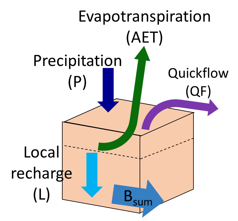
Figure 1. Water balance at the pixel scale to compute the local recharge (Eq. 3), where Bsum is the flow actually reaching the stream.
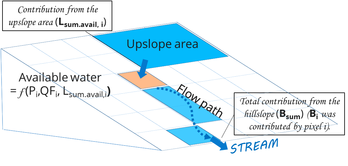
Figure 2. Routing at the hillslope scale to compute actual evapotranspiration (based on each pixel’s climate variables and the upslope contribution, see Eq. 5) and baseflow (based on Bsum, the flow actually reaching the stream, see Eq. 11-14)
Baseflow
The baseflow index represents the contribution of a pixel to baseflow (i.e. water that reaches the stream during the dry season). If the local recharge is negative, then the pixel did not contribute to baseflow so \(B\) is set to zero. If the pixel contributed to groundwater recharge, then \(B\) is a function of the amount of flow leaving the pixel and of the relative contribution to recharge of this pixel.
For a pixel that is not adjacent to the stream channel, the cumulative baseflow, \(B_{sum,i}\), is proportional to the cumulative baseflow leaving the adjacent downslope pixels minus the cumulative baseflow that was generated on that same downslope pixel (Figure 2):
At the watershed outlet (or at any pixel adjacent to the stream), the sum of baseflow generation \(B_{sum,i}\) over all upslope pixels is equal to the sum of local generation over the same pixels (because there is no further opportunity for the slow flow to be consumed before reaching the stream):
where \(L_{sum,i}\) is the cumulative upstream recharge defined by
and the baseflow, \(B_{i}\) can be directly derived from the proportion of the cumulative baseflow leaving cell i, with respect to the available recharge to the upstream cumulative recharge:
Limitations
Like all InVEST models, Seasonal Water Yield uses a simplified approach to estimating quickflow and baseflow, and does not include many of the complexities that occur as water moves through a landscape. Quickflow is primarily based on curve number, which does not take topography into account. For baseflow, although the model uses a physics-based approach, the equations are extremely simplified at both spatial and temporal scales, which significantly increases the uncertainty on the absolute numbers produced. So we do not suggest to use the absolute values, but instead the relative values across the landscapes (where we assume that the simplifications matter less, because they apply to the entire landscape).
Calibration
It is always recommended to validate against observed data if possible. However, while the quickflow output from the model may be used as a quantitative measure, baseflow is intended to be used as an index, not an absolute value. So it is difficult to combine quickflow and baseflow and expect to get realistic model results for validating against observed flow. One possibility is to validate the relative values (i.e. the distribution of values across the landscape). This requires several (at least >3, more realistically >5) stream gauges, which can be compared with the quickflow and baseflow outputs of the model, aggregated to the same stream gauge points. Alternatively, results may be compared to a different spatially-explicit model, if it is available.
If you do try quantitatively validating either quickflow, or a combination of quickflow and baseflow (again, not recommended, but people do try), note that since the results are in millimeters, if we simply sum these up over the whole area, the result is likely to be orders of magnitude too large, and doesn’t represent the total water volume properly. Instead, use the mean B or Qf value across the watershed, convert millimeters to meters, then multiply by the watershed area to get a value in cubic meters, which can be compared against observed flow data. Alternatively, you could calculate volume per pixel and sum those.
Data needs
Raster inputs may have different cell sizes, and they will be resampled to match the cell size of the DEM. Therefore, all model results will have the same cell size as the DEM.
Workspace (required). Folder where model outputs will be written. Make sure that there is ample disk space, and write permissions are correct.
Suffix (optional). Text string that will be appended to the end of output file names, as “_Suffix”. Use a Suffix to differentiate model runs, for example by providing a short name for each scenario. If a Suffix is not provided, or changed between model runs, the tool will overwrite previous results.
Precipitation Directory (required). Folder containing 12 rasters of monthly precipitation for each pixel. Raster file names must end with the month number (e.g. Precip_1.tif for January.) Only .tif files should be in this folder (no .tfw, .xml, etc files). [units: millimeters]
ET0 directory (required). Folder containing 12 rasters of monthly reference evapotranspiration for each pixel. Raster file names must end with the month number (e.g. ET0_1.tif for January.) Only .tif files should be in this folder (no .tfw, .xml, etc files). [units: millimeters]
Digital Elevation Model (required). Raster of elevation for each pixel. Floating point or integer values. [units: meters]
Land use/land cover (required). Raster of land use/land cover (LULC) for each pixel, where each unique integer represents a different land use/land cover class. All values in this raster MUST have corresponding entries in the Biophysical table.
Soil group (required). Raster of SCS soil hydrologic groups (A, B, C, or D), used in combination with the LULC map to compute the curve number (CN) raster. This is a raster of integers where values are entered as numbers 1, 2, 3, and 4, corresponding to soil groups A, B, C, and D, respectively. No other numbers other than 1-4 are allowed, See Appendix 1 for more information.
AOI/Watershed (required). Shapefile delineating the boundary of the watershed to be modeled. Results will be aggregated within each polygon defined. The column ws_id is required, containing a unique integer value for each polygon.
Biophysical table (required). A .csv (Comma Separated Value) table containing model information corresponding to each of the land use classes in the LULC raster. All LULC classes in the LULC raster MUST have corresponding values in this table. Each row is a land use/land cover class and columns must be named and defined as follows:
lucode (required). Unique integer for each LULC class (e.g., 1 for forest, 3 for grassland, etc.) Every value in the LULC map MUST have a corresponding lucode value in the biophysical table.
CN_A, CN_B, CN_C, CN_D (required). Integer curve number (CN) values for each combination of soil type and lucode class. No 0s (zeroes) are allowed.
Kc_1, Kc_2… Kc_11, Kc_12 (required). Floating point monthly crop/vegetation coefficient (Kc) values for each lucode. Kc_1 corresponds to January, Kc_2 February, etc.
Rain events table (either this or a Climate Zone table is required). CSV (comma-separated value, .csv) table with 12 values of rain events, one per month. A rain event is defined as >0.1mm. The following fields are required:
month (required). Values are the integer numbers 1 through 12, corresponding to January (1) through December (12)
events (required). The number of rain events for that month, which are floating point or integer values
Threshold flow accumulation (required). The number of upstream cells that must flow into a cell before it is considered part of a stream, which is used to create streams from the DEM. Smaller values create more tributaries, larger values create fewer. Integer value. See Appendix 1 for more information on choosing this value. Integer value, with no commas or periods - for example “1000”.
alpha_m, beta_i, gamma (required). Model parameters used for research and calibration purposes. Default values are: alpha_m = 1/12, beta_i = 1, gamma = 1. alpha_m is type string; beta_i and gamma are type floating point.
Advanced model options
One model input is the number of rain events per month, which is entered as a .csv table with one number for each month of the year. This assumes that there is one such number for the whole watershed, which may not be true for large areas or areas with very spatially variable precipitation.
To represent variability in the number of rain events, it is possible to enter a map of climate zones, and associated number of rain events for each zone.
Inputs
Climate zone table (either this or a Rain Events table is required). CSV (comma-separated value, .csv) table with the number of rain events per month and climate zone, with the following required fields:
cz_id. Climate zone numbers, integers which correspond to values found in the Climate zone raster
jan feb mar apr may jun jul aug sep oct nov dec. 12 fields corresponding to each month of the year. These contain the number of rain events that occur in that month in that climate zone. Floating point.
Climate zone. Raster of climate zones, each uniquely identified by an integer (i.e. all pixels that are part of one climate zone should have the same integer value.) Must match cz_id values in the Climate zone table.
The model computes sequentially the local recharge layer, and then the baseflow layer from local recharge. Instead of InVEST calculating local recharge, this layer could be obtained from a different model (e.g, RHESSys.) To compute baseflow contribution based on your own recharge layer, it is possible to bypass the first part of the model and directly enter a map of local recharge.
Inputs
Local recharge. Raster with the local recharge obtained from a different model (in mm). Floating point values.
The alpha parameter represents the temporal variability in the contribution of upslope available water to evapotranspiration on a pixel. In the default parameterization, its value is set to 1/12, assuming that the soil buffers water release and that the monthly contribution is exactly 1\12th of the annual contribution.
To allow upslope subsidy to be temporally variable instead, the user can enter monthly alpha values, in the same table as the rain events table.
Inputs
Rain events table. The rain events table is a CSV (comma-separated value, .csv) model input (see above). Along with the required month field, one additional column named alpha is required to run this advanced option. Values for alpha are floating point.
Interpreting outputs
The resolution of the output rasters will be the same as the resolution of the DEM that is provided as input.
[Workspace] folder:
Parameter log: Each time the model is run, a text (.txt) file will be created in the Workspace. The file will list the parameter values and output messages for that run and will be named according to the service, the date and time. When contacting NatCap about errors in a model run, please include the parameter log.
B_[Suffix].tif (type: raster; units: mm, but should be interpreted as relative values, not absolute): Map of baseflow \(B\) values, the contribution of a pixel to slow release flow (which is not evapotranspired before it reaches the stream)
B_sum_[Suffix].tif (type: raster; units: mm, but should be interpreted as relative values, not absolute): Map of \(B_{\text{sum}}\)values, the flow through a pixel, contributed by all upslope pixels, that is not evapotranspirated before it reaches the stream
CN_[Suffix].tif (type: raster): Map of curve number values
L_avail_[Suffix].tif (type: raster; units: mm, but should be interpreted as relative values, not absolute): Map of available local recharge \(L_{\text{avail}}\)
L_[Suffix].tif (type: raster; units: mm, but should be interpreted as relative values, not absolute): Map of local recharge \(L\) values
L_sum_avail_[Suffix].tif (type: raster; units: mm, but should be interpreted as relative values, not absolute): Map of \(L_{\text{sum.avail}}\) values, the available water to a pixel, contributed by all upslope pixels, that is available for evapotranspiration by this pixel
L_sum_[Suffix].tif (type: raster; units: mm, but should be interpreted as relative values, not absolute): Map of \(L_{\text{sum}}\) values, the flow through a pixel, contributed by all upslope pixels, that is available for evapotranspiration to downslope pixels
QF_[Suffix].tif (type: raster; units: mm): Map of quickflow (QF) values
Vri_[Suffix].tif (type: raster; units: mm): Map of the values of recharge (contribution, positive or negative), to the total recharge
aggregated_results_swy_[Suffix].shp: Table containing biophysical values for each watershed, with fields as follows:
qb (units: mm, but should be interpreted as relative values, not absolute): Mean local recharge value within the watershed
[Workspace]\intermediate_outputs folder:
aet_[Suffix].tif (type: raster; units: mm): Map of actual evapotranspiration (AET)
qf_1_[Suffix].tif…qf_12_[Suffix].tif (type: raster; units: mm): Maps of monthly quickflow (1 = January… 12 = December)
stream_[Suffix].tif (type: raster): Stream network generated from the input DEM and Threshold Flow Accumulation. Values of 1 represent streams, values of 0 are non-stream pixels.
Appendix 1: Data sources and guidance for parameter selection
Precipitation
Evapotranspiration
Digital Elevation Model
Land Use/Land Cover
Soil Groups
Watersheds
Curve Number
Kc
Rain Events
Threshold Flow Accumulation
Climate Zones
Climate zone data is available on the Köppen-Geiger climate classification site.
alpha_m
Default: 1/12. See Appendix 2
beta_i
Default: 1. See Appendix 2
gamma
Default: 1. See Appendix 2
Appendix 2: \({\mathbf{\alpha},\mathbf{\beta}}_{\mathbf{i}},\)and \(gamma\) parameters definition and alternative values
\(\alpha\) and \(\beta_{i}\) represent the fraction of annual recharge from upslope pixels that is available to a downslope pixel for evapotranspiration in a given month. The product \(\alpha \times \beta_{i}\) is expected to be <1 since some water from upslope may be unavailable, either when it follows deep flowpaths or when the timing of supply and (evapotranspiration) demand is not synchronized.
\(\alpha\) is a function of precipitation seasonality: recharge from a given month can be used by downslope areas during later months, depending on the subsurface travel times. In the default parameterization, its value is set to 1/12, assuming that the soil buffers water release and that the monthly contribution is exactly one 12th of the annual contribution. An alternative assumption is to set values to the antecedent monthly precipitation values, relative to the total precipitation: Pm-1/Pannual
\(\beta_{i}\) is a function of local topography and soils: for a given amount of upslope recharge, the amount of water used by a pixel is a function of the storage capacity. It also depends on the characteristics of the upslope area: the use of the upslope subsidy is conditioned by the shape and area of the contribution area (i.e. the recharge from the pixel just above the pixel of interest is less likely to be lost than the pixels much further away)
In the default parameterization, \(\beta\) is set to 1 for all pixels. One alternative is to set \(\beta_{i}\) as TI, the topographic wetness index for a pixel, defined as \(ln(\frac{A}{\text{tan}\beta}\)) (or other formulation including soil type and depth).
γ represents the fraction of pixel recharge that is available to downslope pixels. It is a function of soil properties and possibly topography. In the default parameterization, γ is constant over the landscape and plays a role similar to \(\alpha\).
In practice
The options above are provided mainly for research purposes. In practice, we suggest that for highly seasonal climates, alpha should be set to the antecedent monthly precipitation values, relative to the total precipitation: Pm-1/Pannual
Then, we offer two options to address the uncertainty around the parameter values:
Verification of actual evapotranspiration with observations
The model outputs the actual evapotranspiration at the annual time scale: users can adjust parameters to meet observed actual evapotranspiration (e.g. from MODIS, https://www.ntsg.umt.edu/project/modis/mod16.php). In the following, “_mod” stands for modeled AET, “_obs” stands for observed AET.
If AET_mod > AET_obs, the model overpredicts evapotranspiration, which can be corrected by: reducing Kc values, or reducing gamma values, and/or beta values (so less water is available for each pixel).
If AET_mod < AET_obs, the model underpredicts evapotranspiration, which can be corrected by: increasing Kc values (and increasing gamma or beta values if they are not at their maximum of 1).
If monthly values of AET are available, a finer calibration can be performed by changing the seasonal parameter alpha.
Ensemble modeling
The model can be run under different assumptions and the outputs compared to estimate the effect of parameter error. Parameter ranges can be determined from assumptions about the proportion of upslope subsidy available to a given pixel; they can be set to the maximum bounds (0 and 1) for preliminary results.
References
Allen, R.G., Pereira, L.S., Raes, D., Smith, M., 1998. Crop evapotranspiration - Guidelines for computing crop water requirements, FAO Irrigation and drainage paper 56. Rome, Italy.
NRCS-USDA, 2007. National Engineering Handbook. United States Department of Agriculture, https://www.nrcs.usda.gov/wps/portal/nrcs/detailfull/national/water/?cid=stelprdb1043063.