Regression tree#
A regression tree is a type of decision tree used for solving regression problems. Regression problems involve predicting a continuous target variable, as opposed to classification problems where the goal is to predict discrete class labels. Regression trees are a popular machine learning technique for modeling relationships between input features and continuous outcomes.
Here are the key characteristics and concepts related to regression trees:
Decision Tree Structure:
Like classification trees, regression trees are hierarchical structures consisting of nodes. The tree starts with a root node and branches into internal nodes, which in turn branch into leaf nodes (also known as terminal nodes).
Node Splitting:
At each internal node, the tree algorithm selects a feature and a splitting criterion to divide the data into two or more child nodes. The goal is to create splits that minimize the variance of the target variable within each node.
Leaf Nodes:
The leaf nodes are the terminal nodes of the tree. Each leaf node contains a predicted continuous value, which is typically the mean or median of the target values of the training samples in that node.
Predictive Modeling:
To make predictions for new data, you traverse the tree from the root to a leaf node based on the feature values of the new data point. The value in the selected leaf node is the predicted continuous output.
Recursive Partitioning:
The process of building a regression tree is recursive. The algorithm starts with the entire dataset and recursively splits it into subsets by choosing the best feature and split criterion at each node, continuing until a stopping condition is met.
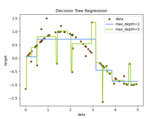
Stopping Criteria:
Stopping criteria are used to determine when to stop growing the tree. Common stopping criteria include limiting the tree depth, setting a minimum number of samples per leaf, or using a minimum impurity reduction threshold.
Impurity Measures:
In regression trees, impurity measures such as Mean Squared Error (MSE) or Mean Absolute Error (MAE) are used to evaluate how well a split reduces the variance of the target variable. The split that minimizes the impurity is selected.
Pruning:
After building a regression tree, it may be pruned to reduce overfitting. Pruning involves removing nodes that do not significantly improve the tree’s performance on a validation dataset.
Visualization:
Regression trees can be visualized graphically, making it easy to interpret and understand the model’s decision-making process.
Ensemble Methods:
Regression trees are often used as building blocks in ensemble methods like Random Forests and Gradient Boosting, which combine multiple trees to improve predictive accuracy and reduce overfitting.
Advantages:
Regression trees are interpretable, can capture complex nonlinear relationships, and are relatively easy to implement. They are useful when the relationship between features and the target variable is non-linear and may have interactions.
Limitations:
They can be prone to overfitting, especially if the tree is allowed to grow deep. Single trees may not generalize well on certain types of data. Ensembling methods like Random Forests and Gradient Boosting can mitigate these limitations.
Regression trees are a valuable tool in machine learning and data analysis, particularly when dealing with regression tasks that require capturing complex relationships between input features and continuous outcomes. Proper tuning of hyperparameters and consideration of potential overfitting are essential when working with regression trees.
Python implementation#
Decision trees can also be applied to regression problems, using the DecisionTreeRegressor class.
As in the classification setting, the fit method will take as argument arrays X and y, only that in this case y is expected to have floating point values instead of integer values:
from sklearn import tree
X = [[0, 0], [2, 2]]
y = [0.5, 2.5]
clf = tree.DecisionTreeRegressor()
clf = clf.fit(X, y)
clf.predict([[1, 1]])
array([0.5])