![]()
from IPython.core.magic import register_cell_magic,register_line_cell_magic
from IPython.display import Javascript, display
import json
display(Javascript(
"""
deleteCell = function() {
var me = document.currentScript;
me.parentElement.parentElement.remove();
};
deleteOutput= function(){
var me = document.currentScript;
me.parentElement.remove();
};
deleteInput = function(){
var me = document.currentScript;
me.parentElement.parentElement.childNodes[1].remove();
};
"""))
@register_line_cell_magic
def deleteCell(*arg):
display(Javascript('deleteCell();'))
@register_line_cell_magic
def deleteOutput(*arg):
display(Javascript('deleteOutput();'))
@register_line_cell_magic
def deleteInput(*arg):
display(Javascript('deleteInput();'))
%deleteInput
%deleteCell
# @title Установка либ { display-mode: "both" }
!pip install jupyterquiz
!pip install matplotlib
!pip install myst_nb
%pip install plotly numpy ipywidgets
zsh:1: command not found: pip
zsh:1: command not found: pip
zsh:1: command not found: pip
Defaulting to user installation because normal site-packages is not writeable
Requirement already satisfied: plotly in /Users/aidarkudabaev/Library/Python/3.9/lib/python/site-packages (5.18.0)
Requirement already satisfied: numpy in /Users/aidarkudabaev/Library/Python/3.9/lib/python/site-packages (1.26.2)
Requirement already satisfied: ipywidgets in /Users/aidarkudabaev/Library/Python/3.9/lib/python/site-packages (8.1.1)
Requirement already satisfied: packaging in /Users/aidarkudabaev/Library/Python/3.9/lib/python/site-packages (from plotly) (23.2)
Requirement already satisfied: tenacity>=6.2.0 in /Users/aidarkudabaev/Library/Python/3.9/lib/python/site-packages (from plotly) (8.2.3)
Requirement already satisfied: comm>=0.1.3 in /Users/aidarkudabaev/Library/Python/3.9/lib/python/site-packages (from ipywidgets) (0.2.0)
Requirement already satisfied: jupyterlab-widgets~=3.0.9 in /Users/aidarkudabaev/Library/Python/3.9/lib/python/site-packages (from ipywidgets) (3.0.9)
Requirement already satisfied: ipython>=6.1.0 in /Users/aidarkudabaev/Library/Python/3.9/lib/python/site-packages (from ipywidgets) (8.18.1)
Requirement already satisfied: traitlets>=4.3.1 in /Users/aidarkudabaev/Library/Python/3.9/lib/python/site-packages (from ipywidgets) (5.14.0)
Requirement already satisfied: widgetsnbextension~=4.0.9 in /Users/aidarkudabaev/Library/Python/3.9/lib/python/site-packages (from ipywidgets) (4.0.9)
Requirement already satisfied: typing-extensions in /Users/aidarkudabaev/Library/Python/3.9/lib/python/site-packages (from ipython>=6.1.0->ipywidgets) (4.8.0)
Requirement already satisfied: pygments>=2.4.0 in /Users/aidarkudabaev/Library/Python/3.9/lib/python/site-packages (from ipython>=6.1.0->ipywidgets) (2.17.2)
Requirement already satisfied: stack-data in /Users/aidarkudabaev/Library/Python/3.9/lib/python/site-packages (from ipython>=6.1.0->ipywidgets) (0.6.3)
Requirement already satisfied: jedi>=0.16 in /Users/aidarkudabaev/Library/Python/3.9/lib/python/site-packages (from ipython>=6.1.0->ipywidgets) (0.19.1)
Requirement already satisfied: matplotlib-inline in /Users/aidarkudabaev/Library/Python/3.9/lib/python/site-packages (from ipython>=6.1.0->ipywidgets) (0.1.6)
Requirement already satisfied: pexpect>4.3 in /Users/aidarkudabaev/Library/Python/3.9/lib/python/site-packages (from ipython>=6.1.0->ipywidgets) (4.9.0)
Requirement already satisfied: prompt-toolkit<3.1.0,>=3.0.41 in /Users/aidarkudabaev/Library/Python/3.9/lib/python/site-packages (from ipython>=6.1.0->ipywidgets) (3.0.41)
Requirement already satisfied: exceptiongroup in /Users/aidarkudabaev/Library/Python/3.9/lib/python/site-packages (from ipython>=6.1.0->ipywidgets) (1.2.0)
Requirement already satisfied: decorator in /Users/aidarkudabaev/Library/Python/3.9/lib/python/site-packages (from ipython>=6.1.0->ipywidgets) (5.1.1)
Requirement already satisfied: parso<0.9.0,>=0.8.3 in /Users/aidarkudabaev/Library/Python/3.9/lib/python/site-packages (from jedi>=0.16->ipython>=6.1.0->ipywidgets) (0.8.3)
Requirement already satisfied: ptyprocess>=0.5 in /Users/aidarkudabaev/Library/Python/3.9/lib/python/site-packages (from pexpect>4.3->ipython>=6.1.0->ipywidgets) (0.7.0)
Requirement already satisfied: wcwidth in /Users/aidarkudabaev/Library/Python/3.9/lib/python/site-packages (from prompt-toolkit<3.1.0,>=3.0.41->ipython>=6.1.0->ipywidgets) (0.2.12)
Requirement already satisfied: executing>=1.2.0 in /Users/aidarkudabaev/Library/Python/3.9/lib/python/site-packages (from stack-data->ipython>=6.1.0->ipywidgets) (2.0.1)
Requirement already satisfied: asttokens>=2.1.0 in /Users/aidarkudabaev/Library/Python/3.9/lib/python/site-packages (from stack-data->ipython>=6.1.0->ipywidgets) (2.4.1)
Requirement already satisfied: pure-eval in /Users/aidarkudabaev/Library/Python/3.9/lib/python/site-packages (from stack-data->ipython>=6.1.0->ipywidgets) (0.2.2)
Requirement already satisfied: six>=1.12.0 in /Library/Developer/CommandLineTools/Library/Frameworks/Python3.framework/Versions/3.9/lib/python3.9/site-packages (from asttokens>=2.1.0->stack-data->ipython>=6.1.0->ipywidgets) (1.15.0)
WARNING: You are using pip version 21.2.4; however, version 23.3.1 is available.
You should consider upgrading via the '/Library/Developer/CommandLineTools/usr/bin/python3 -m pip install --upgrade pip' command.
Note: you may need to restart the kernel to use updated packages.
Newton’s method#
Introduction#
This chapter covers Newton’s method, starting with its definition and application in solving problems, then detailing the basic steps for finding roots. It later continues with an in-depth exploration of the method.
The problem#
Computers are fantastic at crunching numbers and executing algorithms, but analytical solutions to equations often involve symbolic manipulation and reasoning that can be complex. Some equations don’t have closed-form solutions, meaning their solutions can’t be expressed using a finite number of basic mathematical operations and functions.
For example, consider the equation \(x^5 - x + 1 = 0\). This equation doesn’t have a simple analytical solution using elementary functions. In such cases, numerical methods come to the rescue. Computers can iteratively approach the solution with numerical techniques, providing approximate answers.
In essence, computers excel at finding numerical solutions efficiently, but analytical solutions may be elusive for certain types of equations.
Linear Approximations#
Newton’s method, also known as the Newton-Raphson method, is a numerical method intended for approximating the roots or zeros of a function. There are several versions of the method, we will start with the most basic one – the version that iteratively uses a tangent line of a function to approximate the roots.
This basic version of Newton’s Method has a high convergence speed, especially when the initial guess is already a close approximate to the root of the function. However, this version might be sensitive to the choice of initial guess. It can also fail converging if the initial approximation is close to the singular points of a function.
Linear Approximations are widely used in numerical methods to solve equations, and for optimization. This method is applied in engineering, physics, economics, computer science and other fields.
Here is basic usage of this method
def newton_method(func, func_derivative, initial_guess, tol=1e-6, max_iter=100):
x = initial_guess
for iteration in range(max_iter):
f_x = func(x)
f_prime_x = func_derivative(x)
# Avoid division by zero
if abs(f_prime_x) < tol:
raise ValueError("Derivative is close to zero. Newton's method may not converge.")
# Newton's method update
x = x - f_x / f_prime_x
print(f"Current approximation root: {x}")
# Check for convergence
if abs(f_x) < tol:
return x, iteration + 1
raise ValueError("Newton's method did not converge within the maximum number of iterations.")
# Example usage:
def example_function(x):
return x**2 - 4
def example_derivative(x):
return 2 * x
initial_guess = 52
root, num_iter = newton_method(example_function, example_derivative, initial_guess)
print(f"Approximate root: {root}")
print(f"Number of iterations: {num_iter}")
Current approximation root: 26.03846153846154
Current approximation root: 13.096040222701967
Current approximation root: 6.700738029591109
Current approximation root: 3.648843599411131
Current approximation root: 2.372540661342378
Current approximation root: 2.0292485070150263
Current approximation root: 2.0002107861998297
Current approximation root: 2.0000000111065352
Current approximation root: 2.0
Approximate root: 2.0
Number of iterations: 9
One Dimensional Newton’s Method#
Newton’s method, also known as the tangent method, provides an efficient way to solve equations numerically. This method allows you to find approximate values of the roots of functions. Here’s how it works:
Selecting an initial guess: Start by choosing an initial guess \(x_0\), which can be any number.
Calculation of function and derivative: Calculate the value of the function at the point \(x_0\) as \(f(x_0)\) and the value of the derivative of the function at this point as \(f'(x_0)\).
Drawing up the equation of a tangent line: The equation of a tangent line at the point \(x_0\) is represented as: \(y = f(x_0) + f'(x_0)(x - x_0)\).
Finding the root of the tangent line equation: Find the root of the tangent line equation, that is, the value of \(x_1\) at which \(f(x_1) = 0\). This value \(x_1\) becomes a new approximation to the root of the function.
Repeat the process: Continue to apply these steps iteratively using formula at each iteration.
Example#
To demonstrate this process, let’s use the function \(f(x)=x^{2}-2\)
For an initial guess we are going to choose \(x_{0}=1.5\), since \(1\) is too small and \(2\) is too large.
The value of the function at \(x_{0}\) equals \(f(x_{0})=f(1.5)=1.5^{2}-2=0.25\) The value of the derivative of the function at \(x_{0}\) equals \(f'(x_{0})=f'(1.5)=2\)
Drawing the equation of a tangent line \(y=f(x_{0})+f'(x_{0})(x-x_{0})=0.25+3(x-1.5)=0.25+3x-4.5=3x-4.25\)
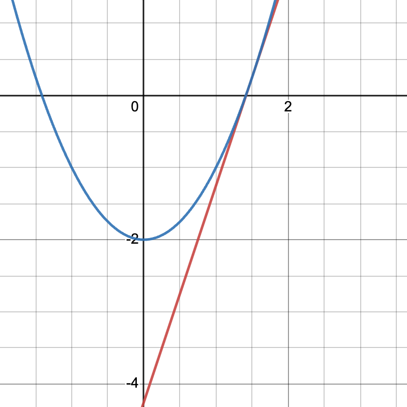
The root of the tangent line equation is \(x=1.416667\), thus the \(x_{1}=1.416667\)
Iterating the process, we get Second iteration:
\(x_{1}=1.416667\), \(f(x_{1})=0.00694539\), \(f'(x_{1})=2.83334\), \(y=2.83334x-4.00695\),
\(x_{2}=1.414214\)
Third iteration:
\(x_{2}=1.414214\), \(f(x_{1})=0.00000124\), \(f'(x_{1})=2.828428\), \(y=2.828428x-4.00000124\),
\(x_{3}=1.414214\)
Now since \(x_{2}=x_{3}\) we can stop the iterating process and conclude that \(x=1.414214\).
Newton’s method converges to the root of the function, providing an exact solution with a sufficiently close initial approximation. This method is widely used in various fields to solve equations.
%deleteInput
from jupyterquiz import display_quiz
quiz = [{
"title": "Quiz: One Dimensional Newton's Method",
"question": "Consider the function $f(x) = x^2 - 4$ with an initial guess $x_0 = 4$. After one iteration of Newton's Method, what is the value of $x_1$?",
"type": "numeric",
"answers": [
{"value": "2.5", "correct": True}
],
"explanation": "Using Newton's Method: $x_1 = x_0 - f(x_0) / f'(x_0)$. Here, $f'(x) = 2x$. So, $x1 = 3 - (4^2 - 4) / (2 * 4) = 2.5$."
}
]
display_quiz(quiz)
Pros and Cons#
Newton’s Method is a powerful tool for finding roots of a function, though besides its advantages it also has some disadvantages too. We will consider the most important notable ones.
Rapid Convergence#
Newton’s method has a quadratic convergence, thus allowing for a rapid root finding process.
Proof for those interested
Based on Taylor’s theorem, a function \(f(x)\) with a continuous second derivative can be represented by an expansion about a point that is close to a root of \(f(x)\). If we suppose that the root is \(α\), then the expansion of \(f(α)\) about \(x_{n}\) is
where \(R_{1}=\frac{1}{2!}{f}''(\xi _{n})(\alpha - x_{n})^{2}\).
Taking into consideration that \(α\) is the root, we get
Further dividing by \({f}'(x_{n})\) gives us
Applying (49), we get
where \(\xi_{n}=\alpha - x_{n}\), thus
And taking the absolute values gives us
Thus, equation (50) shows that the order of convergence is at least quadratic if
\({f}'(x)\neq 0\), for all \(x\in I\) where \(I\) is the interval \(\left [ \alpha - \left | \varepsilon_{0} \right |, \alpha + \left | \varepsilon_{0} \right | \right ]\)
\({f}''(x)\) is continuous, for all \(x \in I\)
\(M\left | \varepsilon_{0} \right |<1\)
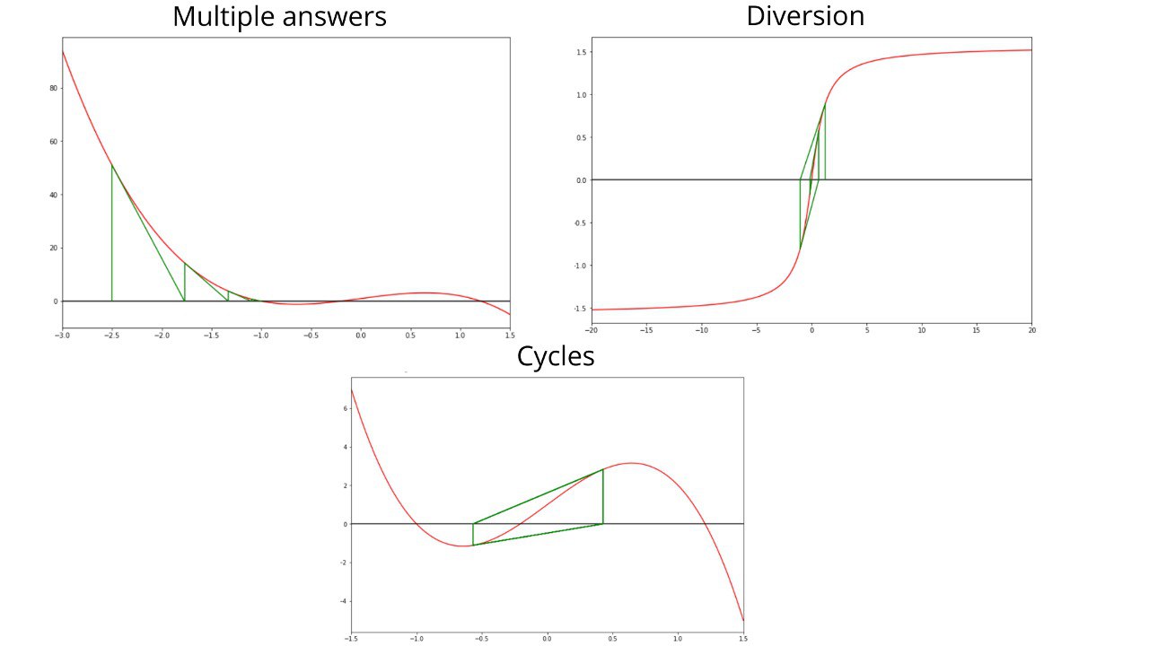
Initial Guess Sensitivity#
Newton’s method might not converge in case if initial guess was a poor estimate.
Proof
For example, let’s consider a function \(f(x)=x^{3}-2x+2\) with a \(0\) as the initial guess. Using the formula (49), we get that \(x_{1}\) is \(1\).
However, the second iteration gives us the value of \(0\) again. So in this case we are stuck in a loop.
Newton’s method continues to be one of the most important tools in numerical analysis and equations solving. Though its application requires careful consideration of the pros and cons in the context of a specific task.
%deleteInput
from jupyterquiz import display_quiz
quiz = [{
"question": "What does Newton's Method primarily use to find the root of a function?",
"type": "multiple_choice",
"answers": [
{
"answer": "First derivative of the function",
"correct": False,
"feedback": ""
},
{
"answer": "Second derivative of the function",
"correct": False,
"feedback": ""
},
{
"answer": "Integral of the function",
"correct": False,
"feedback": ""
},
{
"answer": "Both first and second derivatives of the function",
"correct": True,
"feedback": "Newton's Method uses both the first (for the slope) and second derivatives (for curvature) of the function to find its root."
}
]
}]
display_quiz(quiz)
Newton’s method for optimization#
Generalization for \(d\) dimensions#
Let’s make second order Taylor expansion given \(f:\mathbb{R}^d \rightarrow \mathbb{R}\) to solve optimization problem
\(f(\pmb{x}+\Delta \pmb{x})\approx f(\pmb{x}) + \langle \nabla f(\pmb{x}),\Delta \pmb{x} \rangle+\frac{1}{2}\langle \Delta \pmb{x}, B(\pmb{x})\Delta \pmb{x} \rangle\)
to find minimum, let’s set gradient of above equation to zero
this gives us
\(\Delta \pmb{x} = [B(\pmb{x})]^{-1}\nabla f(\pmb{x})\)
let’s label \(B_k=B(\pmb{x}_k), H_k=B_k^{-1}\)
this gives us iterative Newton’s method step
where \(\nabla f(\pmb{x})\) is called gradient and looks like vector:
and \(B(\pmb{x})\) is called Hessian and looks like matrix:
Note
It can converge to a saddle point instead of to a local minimum
# %% [code]
%deleteInput
import numpy as np
import plotly.graph_objects as go
from myst_nb import glue
# Define the function and its Jacobian (partial derivatives)
def func(x, y):
return x**2 - 2*y**2 + 2
def jac(x, y):
return np.array([2 * x, -4 * y])
def hec():
return np.array([[2, 0], [0, -4]]) # Hessian matrix for this example
# Newton's Method for Multivariate Optimization
def newtons_method(initial_guess, max_iterations=20, tolerance=1e-6, lr=0.01):
x, y = initial_guess
x_vals = [x]
y_vals = [y]
for i in range(max_iterations):
gradient = jac(x, y)
hessian_inv = np.linalg.inv(hec())
update = lr * np.dot(hessian_inv, gradient)
x -= update[0]
y -= update[1]
x_vals.append(x)
y_vals.append(y)
if np.linalg.norm(gradient) < tolerance:
break
return x_vals, y_vals
# Visualize the Optimization Path
initial_guess = np.array([2.0, 2.0])
x_opt, y_opt = newtons_method(initial_guess,lr=0.1)
# Create a surface plot of the function
x_vals = np.linspace(-3, 3, 100)
y_vals = np.linspace(-3, 3, 100)
X, Y = np.meshgrid(x_vals, y_vals)
Z = func(X, Y)
fig = go.Figure(
data=[go.Surface(z=Z, x=X, y=Y, colorscale='Viridis', opacity=0.8)],
layout=go.Layout(
title="Start Title",
updatemenus=[dict(
type="buttons",
buttons=[dict(label="Play",
method="animate",
args=[None])])]
),
frames=[go.Frame(
data=[go.Scatter3d(
x=x_opt[:k+1],
y=y_opt[:k+1],
z=[func(x, y) for x, y in zip(x_opt[:k+1], y_opt[:k+1])],
mode='markers+lines', marker=dict(size=5, color='red')
)],
traces= [0],
name=f'frame{k}'
)for k in range(len(x_opt)-1)]
)
# Add the surface plot
fig.add_trace(go.Surface(z=Z, x=X, y=Y, colorscale='Viridis', opacity=0.8))
# Set layout
fig.update_layout(scene=dict(zaxis=dict(range=[-2, 10])))
fig.update_layout(title="Saddle point")
# Set the backend to notebook for interactive plotting
%matplotlib notebook
fig.show()
Implementation#
Now let’s implement what we learned in the basic form.
import numpy as np
import plotly.graph_objects as go
# Define the function and its Jacobian (partial derivatives)
def func(x, y):
return x**2 + 2*y**2 -2
def jac(x, y):
return np.array([2 * x, 4 * y])
def hess():
return np.array([[2, 0], [0, 4]]) # Hessian matrix for this example
# Newton's Method for Multivariate Optimization
def newtons_method(initial_guess, max_iterations=20, tolerance=1e-6, alpha=0.01):
x, y = initial_guess
x_vals = [x]
y_vals = [y]
for i in range(max_iterations):
gradient = jac(x, y)
hessian_inv = np.linalg.inv(hess())
update = alpha * np.dot(hessian_inv, gradient)
x -= update[0]
y -= update[1]
x_vals.append(x)
y_vals.append(y)
if np.linalg.norm(gradient) < tolerance:
break
return x_vals, y_vals
Note that the method returns an array. To get the final result just print the last element. Here is an example usage of it:
initial_guess = np.array([2.0, 2.0])
x_opt, y_opt = newtons_method(initial_guess,alpha=0.5)
print(f"optimal x:{x_opt[-1]}")
print(f"optimal y:{y_opt[-1]}")
optimal x:1.9073486328125e-06
optimal y:1.9073486328125e-06
You can tweak alpha parameter and max_iterations to test the convergence.
About \(\alpha\)
In literature if \(\alpha \in (0,1)\) then this method is called damped Newton’s method
%deleteInput
# Create a surface plot of the function
x_vals = np.linspace(-3, 3, 100)
y_vals = np.linspace(-3, 3, 100)
x, Y = np.meshgrid(x_vals, y_vals)
Z = func(x, Y)
fig = go.Figure(
data=[go.Surface(z=Z, x=x, y=Y, colorscale='Viridis', opacity=0.8)],
layout=go.Layout(
title="Start Title",
updatemenus=[dict(
type="buttons",
buttons=[dict(label="Play",
method="animate",
args=[None])])]
),
frames=[go.Frame(
data=[go.Scatter3d(
x=x_opt[:k+1],
y=y_opt[:k+1],
z=[func(x, y) for x, y in zip(x_opt[:k+1], y_opt[:k+1])],
mode='markers+lines', marker=dict(size=5, color='red')
)],
traces= [0],
name=f'frame{k}'
)for k in range(len(x_opt)-1)]
)
# Add the surface plot
fig.add_trace(go.Surface(z=Z, x=x, y=Y, colorscale='Viridis', opacity=0.8))
# Set layout
fig.update_layout(scene=dict(zaxis=dict(range=[-2, 10])))
fig.update_layout(title="Newton's Method in 3D")
fig.show()
Application in ML#
Newton’s Method is a very useful tool for the optimization process in Machine Learning. It allows us to adjust several parameters of a model at once, unlike other methods (e.g. Gradient Descent) that only let us adjust one parameter at a time.
In other words, Newton’s Method looks at both the slope and the curvature – first and second derivatives respectively. This can make it much faster in terms of optimization.
However, it is also worth noting that Newton’s Method might be trickier to use when a model is very complex. Thus, we can say that Newton’s Method is quicker but more risky, while Gradient Descent is more steady but slow.
To solve the optimization problem in ML
do the followind steps:
initialize \(\pmb{w}\) by some random values (e.g., from \(\mathcal N(0, 1)\))
choose tolerance \(\varepsilon > 0\) and learning rate \(\eta > 0\)
while \(\Vert \nabla\mathcal L(\pmb{w}) \Vert > \varepsilon\) do the iteration step!
return \(\pmb{w}\)
Carefull!
If condition \(\Vert \nabla\mathcal L(w) \Vert > \varepsilon\) holds for too long, the loop in step 3 terminates after some number iterations max_iter.
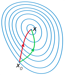
Gradient descent (green) and Newton’s method (red) in comparison for minimizing a function (with small step sizes).
%deleteInput
from jupyterquiz import display_quiz
quiz = [{
"question": "Which of the following is an advantage of Newton's Method?",
"type": "multiple_choice",
"answers": [
{
"answer": "Requires less memory compared to other methods",
"correct": False,
"feedback": "Incorrect, try again"
},
{
"answer": "Typically converges faster than gradient descent for well-behaved functions",
"correct": True,
"feedback": "Newton's Method can converge more quickly for certain types of functions due to its use of both first and second derivatives."
},
{
"answer": "Does not require calculation of second derivatives",
"correct": False,
"feedback": "Incorrect, try again"
},
{
"answer": "Suitable for very large datasets",
"correct": False,
"feedback": "Incorrect, try again"
}
]
}]
display_quiz(quiz)