Regularization#
If the columns of the feature matrix \(\boldsymbol X\) are highly correlated, the weights of linear regression could be unstable and excessively large. To fight this, a regularization term is added to the MSE loss function.
Ridge regression#
To penalize weights that are too large in magnitude, add a multiple of
to RSS; the new loss function is
To find the optimal weights, one need to solve the equation \(\nabla_{\boldsymbol w} \mathcal L(\boldsymbol w) = \boldsymbol 0\).
Since \(\nabla_{\boldsymbol w}(\Vert \boldsymbol w \Vert_2^2) = 2\boldsymbol w\), we receive one additional term to (18):
From here we obtain
Note that this is equal to (19) if \(C=0\). Ridge regression also allows to avoid inverting of a singular matrix.
Once again take the Boston dataset, and try ridge regression on it:
from sklearn.linear_model import Ridge
import numpy as np
import pandas as pd

boston = pd.read_csv("../ISLP_datsets/Boston.csv")

target = boston['medv']
train = boston.drop(['medv', "Unnamed: 0"], axis=1)
ridge = Ridge()
ridge.fit(train, target)
print("intercept:", ridge.intercept_)
print("coefficients:", ridge.coef_)
print("r-score:", ridge.score(train, target))
print("MSE:", np.mean((ridge.predict(train) - target) ** 2))
intercept: 36.66359752181638
coefficients: [-1.18324104e-01  4.80549483e-02 -1.78537994e-02  2.70383610e+00
 -1.14024737e+01  3.70139930e+00 -2.75076805e-03 -1.38242357e+00
  2.71825248e-01 -1.33051618e-02 -8.55687104e-01 -5.62037458e-01]
r-score: 0.73233360340788
MSE: 22.59627839822696
LASSO regression#
The only difference with ridge regression is that \(L^1\)-norm is used for the regularization term:
Accordingly, the loss function switches to
and the optimal weights \(\widehat w\) are the solution of the optimization task
Note
LASSO stands for Least Absolute Shrinkage and Selection Operator
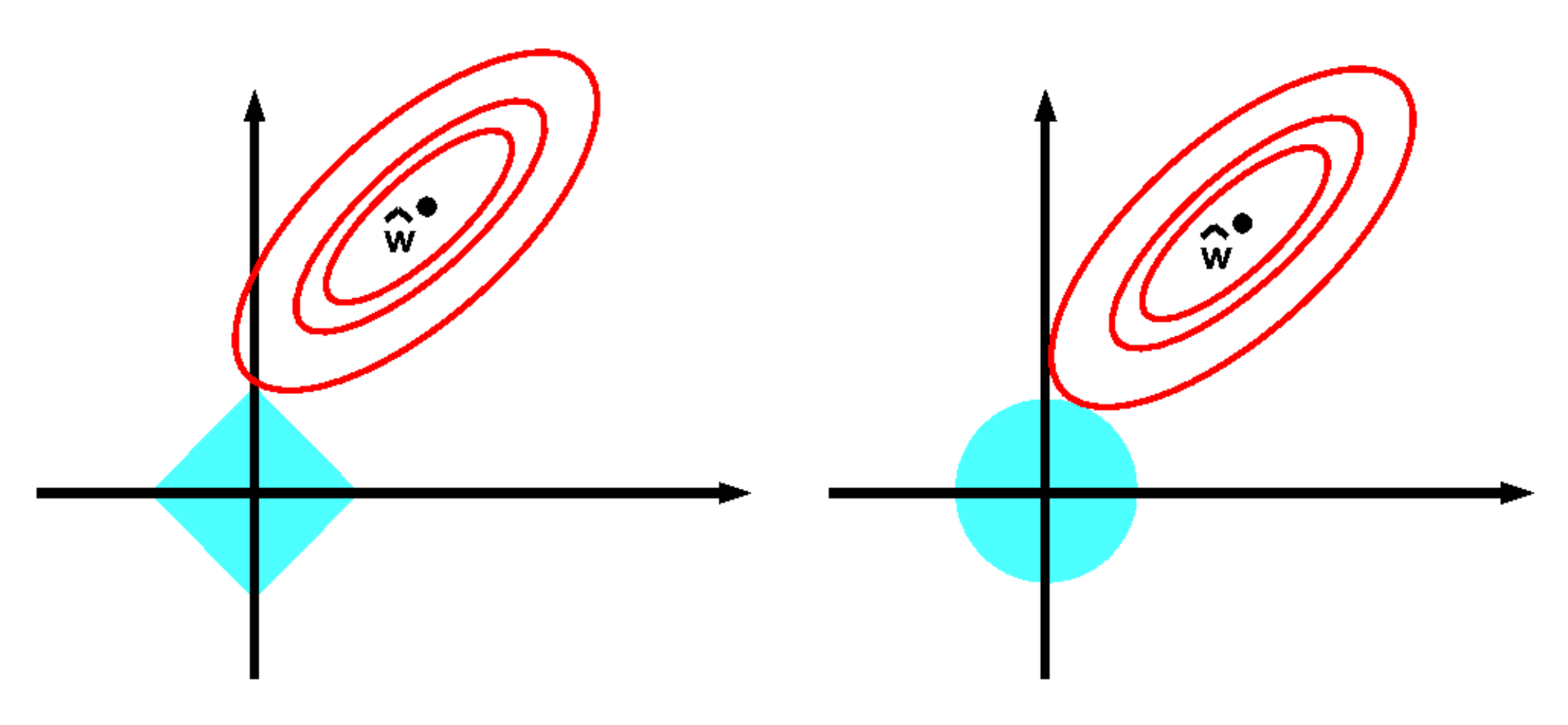
Important property of Lasso regression is feature selection. Usually some coorditates of the optimal vector of weights \(\widehat {\boldsymbol w}\) turn out to be zero. A famous picture from [Murphy, 2022]:
Advantages of LASSO
strong theoretical guarantees
sparse solution
feature selection
However, there is no closed-form solution of (21).
Empirical recipe to provide better prediction performance:
first, perform variable selection using LASSO;
Second, re-estimate model parameters with selected variables using Ridge regression.
See how Lasso regression works on Boston dataset:
from sklearn.linear_model import Lasso

lasso = Lasso()
lasso.fit(train, target)
print("intercept:", lasso.intercept_)
print("coefficients:", lasso.coef_)
print("r-score:", lasso.score(train, target))
print("MSE:", np.mean((lasso.predict(train) - target) ** 2))
intercept: 44.98510958345055
coefficients: [-0.07490856  0.05004565 -0.          0.         -0.          0.83244563
  0.02266242 -0.66083402  0.25070221 -0.01592473 -0.70206981 -0.7874801 ]
r-score: 0.6745576822708007
MSE: 27.47369601713281
Three coeffitients vanished, namely indus, chas, nox:
boston.columns[3:6]
Index(['indus', 'chas', 'nox'], dtype='object')
Elastic net#
Elasitc net is a hybrid between lasso and ridge regression. This corresponds to minimizing the following objective:
Motivation
If there is a group of variables with high pairwise correlations, then the LASSO tends to select only one variable from the group and does not care which one is selected
It has been empirically observed that the prediction performance of the LASSO is dominated by ridge regression
Elastic Net includes regression, variable selection, with the capacity of selecting groups of correlated variables
Elas9tic Net is like a stretchable fishing net that retains ‘all the big fish’ ([Zou and Hastie, 2003])
Applied to Boston dataset, it zeroes two coefficients:
from sklearn.linear_model import ElasticNet

en = ElasticNet()
en.fit(train, target)
print("intercept:", en.intercept_)
print("coefficients:", en.coef_)
print("r-score:", en.score(train, target))
print("MSE:", np.mean((en.predict(train) - target) ** 2))
intercept: 45.68409537995804
coefficients: [-0.09222698  0.05335925 -0.02011639  0.         -0.          0.89077605
  0.02193951 -0.7586982   0.28439842 -0.01686424 -0.72640381 -0.77837394]
r-score: 0.679766219677128
MSE: 27.033993601067873
Exercises#
Prove that the matrix \(\boldsymbol X^\top \boldsymbol X + C\boldsymbol I\) is invertible for all \(C >0\).
TODO
Add some simple quizzes
Add more datasets
Show the advantages of different typse of regularization on real and/or simulated datasets
Describe
Ridge(),Lasso(),ElasticNet()more thoroughly