Classification Metrics#
Classification metrics are used to evaluate the performance of classification models, which are machine learning models that predict categorical labels or classes for input data.
Accuracy#
The most common metric for binary and multiclass classification which shows the fraction of correct predictions:
More formally, if \(\mathcal D = \{(\boldsymbol x_i, y_i)\}_{i=1}^n\) is the train (or test) dataset, then the accuracy metric is defined as follows:
Q. What can be the value of accuracy if \(n=4\)?
Note
The missclassificaton rate (or error rate) (1) is a similar metric and equals to \(1 -\mathrm{acc}\).
Confusion matrix#
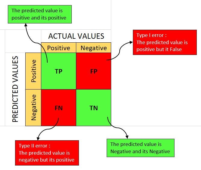
If \(\mathcal Y = \{-1, +1\}\) then there are four possibilites how the prediction \(\widehat y\) of a classifier can relate to the true label \(y\).
Metric |
Prediction \(\widehat y\) |
Ground truth \(y\) |
|---|---|---|
true positive, TP |
\(+1\) |
\(+1\) |
false positive, FP |
\(+1\) |
\(-1\) |
false negative, FN |
\(-1\) |
\(+1\) |
true negative, TN |
\(-1\) |
\(-1\) |
Tip
The first word (true/false) shows whether the prediction is correct. The second one (positive/negative) indicates the predicted label.
These metrics are usually aggregated from the whole dataset \(\mathcal D\), i. e.,
True Positives represent the number of correctly predicted positive instances:
\[ \mathrm{TP} = \sum\limits_{i=1}^n \mathbb I[\widehat y_i = +1, y_i = +1]; \]False Positives represent the number of instances that were actually negative but were predicted as positive:
\[ \mathrm{FP} = \sum\limits_{i=1}^n \mathbb I[\widehat y_i = +1, y_i = -1]; \]False Negatives represent the number of instances that were actually positive but were predicted as negative.
\[ \mathrm{FN} = \sum\limits_{i=1}^n \mathbb I[\widehat y_i = -1, y_i = +1]; \]True Negatives represent the number of correctly predicted negative instances:
Note
If \(\mathcal Y = \{0, 1\}\), then negative class is \(0\), positive class is \(1\).
These four metrics form the confusion matrix.
Q. What is the correct formula for accuracy?
\(\frac{\mathrm{TP}}{\mathrm{TP} + \mathrm{TN} + \mathrm{FP} + \mathrm{FN}}\)
\(\frac{\mathrm{TP} + \mathrm{TN}}{\mathrm{TP} + \mathrm{TN} + \mathrm{FP} + \mathrm{FN}}\)
\(\frac{\mathrm{TP} + \mathrm{FN}}{\mathrm{TP} + \mathrm{TN} + \mathrm{FP} + \mathrm{FN}}\)
\(\frac{\mathrm{TP} + \mathrm{FP}}{\mathrm{TP} + \mathrm{TN} + \mathrm{FP} + \mathrm{FN}}\)
Example: breast cancer dataset#
from sklearn.datasets import load_breast_cancer
data = load_breast_cancer()

# 0 should be "benign"
# 1 should be "malignant"
relabeled_target = 1 - data["target"]

X = data["data"]
y = relabeled_target
data.target_names
array(['malignant', 'benign'], dtype='<U9')
Train logistic regression and print metrics:
from sklearn.linear_model import LogisticRegression
from sklearn.metrics import confusion_matrix
from sklearn.model_selection import train_test_split

X_train, X_test, y_train, y_test = train_test_split(X, y)
log_reg = LogisticRegression(max_iter=3000)
log_reg.fit(X_train, y_train)

print("Train accuracy:", log_reg.score(X_train, y_train))
print("Confusion matrix on train dataset:\n", confusion_matrix(y_train, log_reg.predict(X_train)))
print("Test accuracy:", log_reg.score(X_test, y_test))
print("Confusion matrix on train dataset:\n", confusion_matrix(y_test, log_reg.predict(X_test)))
Train accuracy: 0.9671361502347418
Confusion matrix on train dataset:
 [[261   5]
 [  9 151]]
Test accuracy: 0.9440559440559441
Confusion matrix on train dataset:
 [[88  3]
 [ 5 47]]
For classification into \(K\) classes the confusion matrix has shape \(K\times K\). For example, for MNIST dataset we had \(10\) rows and \(10\) columns.
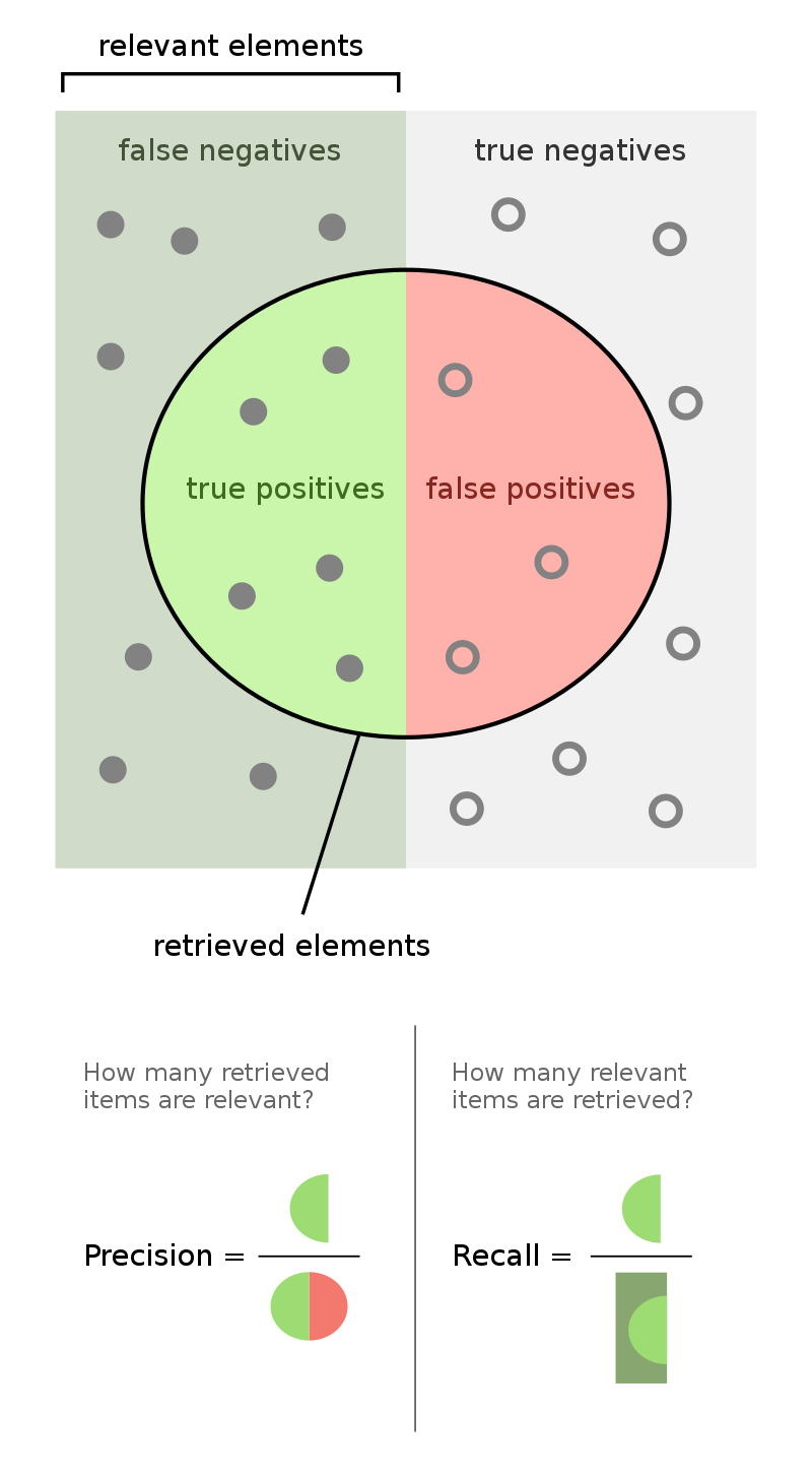
Precision and recall#
Accuracy score is a poor metric if classes are unbalanced. For instance, if \(1\%\) of tested people are really sick, then predicting always negative (i.e., the patient is healthy) would give \(99\%\) of accuracy. Of course, such dummy model is useless in this case.
Precision#
Precision, also known as positive predictive value, measures the proportion of true positive predictions among all positive predictions made by the model:
It is useful when minimizing false positives is a priority.
Recall#
Recall measures the proportion of true positive predictions among all actual positive instances.
It is particularly important when minimizing false negatives is crucial.
Q. Which metric is more relevant in the following cases?
testing on covid-19 or any other dangerous and contagious desease;
a nuclear warning system which makes decision whether to launch nuclear missles in response.
\(F\)-score#
The \(F_1\)-score is the harmonic mean of precision and recall. It provides a balance between precision and recall and is especially useful when there is an imbalance between the classes.
The \(F_\beta\)-score is a generalization of the \(F_1\)-score:
Q. What is happening with \(F_\beta\)-score if \(\beta \to +0\)? \(\beta \to +\infty\)?
Q. Calculate precision, recall and \(F_1\)-score for the data from this table.
Example: imbalanced dataset#
import pandas as pd

credit_df = pd.read_csv("../ISLP_datsets/creditcard.csv.zip")
credit_df.head()
| Time | V1 | V2 | V3 | V4 | V5 | V6 | V7 | V8 | V9 | ... | V21 | V22 | V23 | V24 | V25 | V26 | V27 | V28 | Amount | Class | |
|---|---|---|---|---|---|---|---|---|---|---|---|---|---|---|---|---|---|---|---|---|---|
| 0 | 0.0 | -1.359807 | -0.072781 | 2.536347 | 1.378155 | -0.338321 | 0.462388 | 0.239599 | 0.098698 | 0.363787 | ... | -0.018307 | 0.277838 | -0.110474 | 0.066928 | 0.128539 | -0.189115 | 0.133558 | -0.021053 | 149.62 | 0 |
| 1 | 0.0 | 1.191857 | 0.266151 | 0.166480 | 0.448154 | 0.060018 | -0.082361 | -0.078803 | 0.085102 | -0.255425 | ... | -0.225775 | -0.638672 | 0.101288 | -0.339846 | 0.167170 | 0.125895 | -0.008983 | 0.014724 | 2.69 | 0 |
| 2 | 1.0 | -1.358354 | -1.340163 | 1.773209 | 0.379780 | -0.503198 | 1.800499 | 0.791461 | 0.247676 | -1.514654 | ... | 0.247998 | 0.771679 | 0.909412 | -0.689281 | -0.327642 | -0.139097 | -0.055353 | -0.059752 | 378.66 | 0 |
| 3 | 1.0 | -0.966272 | -0.185226 | 1.792993 | -0.863291 | -0.010309 | 1.247203 | 0.237609 | 0.377436 | -1.387024 | ... | -0.108300 | 0.005274 | -0.190321 | -1.175575 | 0.647376 | -0.221929 | 0.062723 | 0.061458 | 123.50 | 0 |
| 4 | 2.0 | -1.158233 | 0.877737 | 1.548718 | 0.403034 | -0.407193 | 0.095921 | 0.592941 | -0.270533 | 0.817739 | ... | -0.009431 | 0.798278 | -0.137458 | 0.141267 | -0.206010 | 0.502292 | 0.219422 | 0.215153 | 69.99 | 0 |
5 rows × 31 columns
y = credit_df['Class']
X = credit_df.drop("Class", axis=1)
y.value_counts()
Class
0    284315
1       492
Name: count, dtype: int64
An ideal distribution of classes for a dummy model :)
from sklearn.metrics import accuracy_score, precision_score, recall_score, f1_score
from sklearn.model_selection import train_test_split
X_train, X_test, y_train, y_test = train_test_split(X, y)
y_test.value_counts()
Class
0    71077
1      125
Name: count, dtype: int64
from sklearn.dummy import DummyClassifier
dc_mf = DummyClassifier(strategy="most_frequent")
dc_mf.fit(X_train, y_train)
print("Accuracy:", accuracy_score(y_test, dc_mf.predict(X_test)))
print("Precision:", precision_score(y_test, dc_mf.predict(X_test)))
print("Recall:", recall_score(y_test, dc_mf.predict(X_test)))
print("F1 score:", f1_score(y_test, dc_mf.predict(X_test)))
Accuracy: 0.9982444313361984
Precision: 0.0
Recall: 0.0
F1 score: 0.0
/Library/Frameworks/Python.framework/Versions/3.11/lib/python3.11/site-packages/sklearn/metrics/_classification.py:1469: UndefinedMetricWarning: Precision is ill-defined and being set to 0.0 due to no predicted samples. Use `zero_division` parameter to control this behavior.
  _warn_prf(average, modifier, msg_start, len(result))
Let’s try the logistic regression:
from sklearn.linear_model import LogisticRegression

log_reg = LogisticRegression(max_iter=10000)
log_reg.fit(X_train, y_train)
LogisticRegression(max_iter=10000)In a Jupyter environment, please rerun this cell to show the HTML representation or trust the notebook.
On GitHub, the HTML representation is unable to render, please try loading this page with nbviewer.org.
LogisticRegression(max_iter=10000)
print("Accuracy:", accuracy_score(y_test, log_reg.predict(X_test)))
print("Precision:", precision_score(y_test, log_reg.predict(X_test)))
print("Recall:", recall_score(y_test, log_reg.predict(X_test)))
print("F1 score:", f1_score(y_test, log_reg.predict(X_test)))
Accuracy: 0.9992135052386169
Precision: 0.7870370370370371
Recall: 0.7203389830508474
F1 score: 0.752212389380531