Basic Diagnostics
Ann Wells
April 23, 2023
Introduction and Data files
Data and analysis description
This dataset contains nine tissues (heart, hippocampus, hypothalamus, kidney, liver, prefrontal cortex, skeletal muscle, small intestine, and spleen) from C57BL/6J mice that were fed 2-deoxyglucose (6g/L) through their drinking water for 96hrs or 4wks. The organs from the mice were harvested and processed for metabolomics and transcriptomics. The data in this document pertains to the transcriptomics data only. This document specifically only calculates and plots principal component analysis for log transformed data.
needed.packages <- c("tidyverse", "here", "functional", "gplots", "dplyr", "GeneOverlap", "R.utils", "reshape2","magrittr","data.table", "RColorBrewer","preprocessCore","plotly")
for(i in 1:length(needed.packages)){library(needed.packages[i], character.only = TRUE)}
setwd(here("Data","counts"))
files <- dir(pattern = "*.txt")
data <- files %>% map(read_table2) %>% reduce(full_join, by="gene_id")
tdata <- t(sapply(data, as.numeric))
tdata.FPKM <- grep("FPKM", rownames(tdata))
tdata.FPKM <- tdata[tdata.FPKM,]
colnames(tdata.FPKM) <- data$gene_id
tdata.FPKM <-tdata.FPKM[,colSums(tdata.FPKM) > 0]
# Read all the files and create a FileName column to store filenames
DT <- rbindlist(sapply(files, fread, simplify = FALSE),
use.names = TRUE, idcol = "FileName")
name <- strsplit(DT$FileName,"_")
samples <-c()
for(i in 1:length(name)){
samples[[i]] <- as.list(paste(name[[i]][1],name[[i]][2], sep="_"))
}
sampleID <- unique(rapply(samples, function(x) head(x,c(1))))
names <- unique(rapply(name, function(x) head(x,c(1))))
#names.samples <- c(names, names[12], names[14], names[17], names[37], names[41], names[11], names[49])
names.samples <- sort(names)
tdata.FPKM.names.samples <- cbind(names.samples, tdata.FPKM)
rownames(tdata.FPKM.names.samples) <- names
rownames(tdata.FPKM) <- names
#lengthID <- table(sampleID)
sample.info <- read_csv(here("Data","Sample_layout_RNAseq_mouse_ID_B6_96hr_4wk.csv"))
#sample.info.duplicated <- rbind(sample.info[16,], sample.info[17,], sample.info[21,], sample.info[27,], sample.info[54,],
# sample.info[60,], sample.info[70,], sample.info)
#sample.info.duplicated <- sample.info.duplicated %>% arrange(`Sample ID`)
tdata.FPKM.names.samples <- rownames_to_column(as.data.frame(tdata.FPKM.names.samples)) # %>% mutate("Sample ID" = rownames(tdata.FPKM))
tdata.FPKM.sample.info <- left_join(tdata.FPKM.names.samples, sample.info, by = c("names.samples" = "Sample ID"))
rownames(tdata.FPKM.sample.info) <- names
saveRDS(tdata.FPKM.sample.info[,-c(1:2)], here("Data", "20190406_RNAseq_B6_4wk_2DG_counts_phenotypes.RData"))
saveRDS(tdata.FPKM, here("Data", "20190406_RNAseq_B6_4wk_2DG_counts_numeric.RData"))PCA (logged all data)
These plots contain all tissues, treatments, and times.
Scree plot and Summary Statistics
tdata.FPKM.sample.info <- readRDS(here("Data","20190406_RNAseq_B6_4wk_2DG_counts_phenotypes.RData"))

tdata.FPKM <- readRDS(here("Data","20190406_RNAseq_B6_4wk_2DG_counts_numeric.RData"))

log.tdata.FPKM <- log(tdata.FPKM + 1)

pca <- prcomp(log.tdata.FPKM, center = T)

screeplot(pca,type = "lines")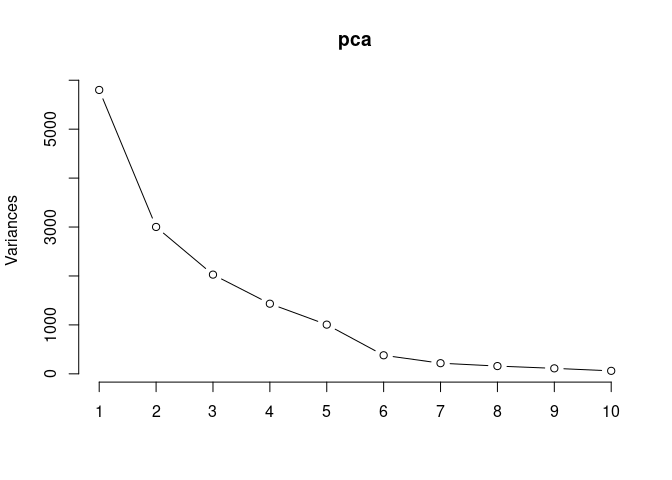
summary(pca)## Importance of components:
## PC1 PC2 PC3 PC4 PC5 PC6
## Standard deviation 76.1635 54.7836 45.0259 37.85276 31.70683 19.46567
## Proportion of Variance 0.3853 0.1994 0.1347 0.09518 0.06678 0.02517
## Cumulative Proportion 0.3853 0.5847 0.7194 0.81455 0.88133 0.90650
## PC7 PC8 PC9 PC10 PC11 PC12
## Standard deviation 14.74359 12.59024 10.57785 7.80441 7.07696 6.95078
## Proportion of Variance 0.01444 0.01053 0.00743 0.00405 0.00333 0.00321
## Cumulative Proportion 0.92094 0.93147 0.93890 0.94295 0.94627 0.94948
## PC13 PC14 PC15 PC16 PC17 PC18 PC19
## Standard deviation 6.28378 5.46547 5.28198 4.95913 4.68720 4.47898 4.43441
## Proportion of Variance 0.00262 0.00198 0.00185 0.00163 0.00146 0.00133 0.00131
## Cumulative Proportion 0.95210 0.95409 0.95594 0.95758 0.95903 0.96037 0.96167
## PC20 PC21 PC22 PC23 PC24 PC25 PC26
## Standard deviation 4.20069 3.94951 3.84179 3.80632 3.59080 3.51619 3.4634
## Proportion of Variance 0.00117 0.00104 0.00098 0.00096 0.00086 0.00082 0.0008
## Cumulative Proportion 0.96285 0.96388 0.96486 0.96582 0.96668 0.96750 0.9683
## PC27 PC28 PC29 PC30 PC31 PC32 PC33
## Standard deviation 3.37579 3.28815 3.2355 3.15927 3.11856 3.04103 3.0012
## Proportion of Variance 0.00076 0.00072 0.0007 0.00066 0.00065 0.00061 0.0006
## Cumulative Proportion 0.96906 0.96977 0.9705 0.97113 0.97178 0.97239 0.9730
## PC34 PC35 PC36 PC37 PC38 PC39 PC40
## Standard deviation 2.97516 2.93892 2.90576 2.83769 2.76670 2.71778 2.64637
## Proportion of Variance 0.00059 0.00057 0.00056 0.00053 0.00051 0.00049 0.00047
## Cumulative Proportion 0.97358 0.97415 0.97471 0.97525 0.97576 0.97625 0.97671
## PC41 PC42 PC43 PC44 PC45 PC46 PC47
## Standard deviation 2.63705 2.59007 2.56309 2.53879 2.47098 2.4397 2.39859
## Proportion of Variance 0.00046 0.00045 0.00044 0.00043 0.00041 0.0004 0.00038
## Cumulative Proportion 0.97718 0.97762 0.97806 0.97849 0.97889 0.9793 0.97967
## PC48 PC49 PC50 PC51 PC52 PC53 PC54
## Standard deviation 2.38243 2.34626 2.31362 2.28793 2.26420 2.24568 2.21255
## Proportion of Variance 0.00038 0.00037 0.00036 0.00035 0.00034 0.00033 0.00033
## Cumulative Proportion 0.98005 0.98041 0.98077 0.98111 0.98146 0.98179 0.98212
## PC55 PC56 PC57 PC58 PC59 PC60 PC61
## Standard deviation 2.19843 2.18029 2.16757 2.16158 2.14731 2.1367 2.1235
## Proportion of Variance 0.00032 0.00032 0.00031 0.00031 0.00031 0.0003 0.0003
## Cumulative Proportion 0.98244 0.98275 0.98306 0.98337 0.98368 0.9840 0.9843
## PC62 PC63 PC64 PC65 PC66 PC67 PC68
## Standard deviation 2.10434 2.09277 2.08540 2.06718 2.04285 2.03913 2.01055
## Proportion of Variance 0.00029 0.00029 0.00029 0.00028 0.00028 0.00028 0.00027
## Cumulative Proportion 0.98458 0.98487 0.98516 0.98544 0.98572 0.98600 0.98626
## PC69 PC70 PC71 PC72 PC73 PC74 PC75
## Standard deviation 2.00888 1.99009 1.96810 1.95476 1.94505 1.92616 1.91976
## Proportion of Variance 0.00027 0.00026 0.00026 0.00025 0.00025 0.00025 0.00024
## Cumulative Proportion 0.98653 0.98679 0.98705 0.98731 0.98756 0.98780 0.98805
## PC76 PC77 PC78 PC79 PC80 PC81 PC82
## Standard deviation 1.91023 1.90834 1.89879 1.88164 1.86859 1.85571 1.85011
## Proportion of Variance 0.00024 0.00024 0.00024 0.00024 0.00023 0.00023 0.00023
## Cumulative Proportion 0.98829 0.98853 0.98877 0.98901 0.98924 0.98947 0.98970
## PC83 PC84 PC85 PC86 PC87 PC88 PC89
## Standard deviation 1.83943 1.83095 1.82698 1.81985 1.80865 1.80483 1.79055
## Proportion of Variance 0.00022 0.00022 0.00022 0.00022 0.00022 0.00022 0.00021
## Cumulative Proportion 0.98992 0.99014 0.99036 0.99058 0.99080 0.99102 0.99123
## PC90 PC91 PC92 PC93 PC94 PC95 PC96
## Standard deviation 1.77195 1.76848 1.76312 1.7544 1.7398 1.7350 1.7297
## Proportion of Variance 0.00021 0.00021 0.00021 0.0002 0.0002 0.0002 0.0002
## Cumulative Proportion 0.99144 0.99165 0.99185 0.9921 0.9923 0.9925 0.9927
## PC97 PC98 PC99 PC100 PC101 PC102 PC103
## Standard deviation 1.7247 1.7174 1.71018 1.69784 1.69030 1.67473 1.66483
## Proportion of Variance 0.0002 0.0002 0.00019 0.00019 0.00019 0.00019 0.00018
## Cumulative Proportion 0.9929 0.9930 0.99325 0.99344 0.99363 0.99381 0.99400
## PC104 PC105 PC106 PC107 PC108 PC109 PC110
## Standard deviation 1.65542 1.64970 1.63902 1.63612 1.62606 1.62111 1.60370
## Proportion of Variance 0.00018 0.00018 0.00018 0.00018 0.00018 0.00017 0.00017
## Cumulative Proportion 0.99418 0.99436 0.99454 0.99472 0.99489 0.99507 0.99524
## PC111 PC112 PC113 PC114 PC115 PC116 PC117
## Standard deviation 1.59944 1.59487 1.58698 1.57751 1.56975 1.56400 1.56180
## Proportion of Variance 0.00017 0.00017 0.00017 0.00017 0.00016 0.00016 0.00016
## Cumulative Proportion 0.99541 0.99558 0.99574 0.99591 0.99607 0.99624 0.99640
## PC118 PC119 PC120 PC121 PC122 PC123 PC124
## Standard deviation 1.54983 1.54450 1.52332 1.52185 1.52163 1.51328 1.50233
## Proportion of Variance 0.00016 0.00016 0.00015 0.00015 0.00015 0.00015 0.00015
## Cumulative Proportion 0.99656 0.99672 0.99687 0.99702 0.99718 0.99733 0.99748
## PC125 PC126 PC127 PC128 PC129 PC130 PC131
## Standard deviation 1.49612 1.48793 1.48198 1.47861 1.46557 1.45659 1.44221
## Proportion of Variance 0.00015 0.00015 0.00015 0.00015 0.00014 0.00014 0.00014
## Cumulative Proportion 0.99763 0.99778 0.99792 0.99807 0.99821 0.99835 0.99849
## PC132 PC133 PC134 PC135 PC136 PC137 PC138
## Standard deviation 1.43984 1.42774 1.42078 1.40564 1.40366 1.39370 1.38077
## Proportion of Variance 0.00014 0.00014 0.00013 0.00013 0.00013 0.00013 0.00013
## Cumulative Proportion 0.99863 0.99876 0.99890 0.99903 0.99916 0.99929 0.99941
## PC139 PC140 PC141 PC142 PC143 PC144
## Standard deviation 1.37164 1.35793 1.34902 1.30094 1.26209 1.481e-14
## Proportion of Variance 0.00012 0.00012 0.00012 0.00011 0.00011 0.000e+00
## Cumulative Proportion 0.99954 0.99966 0.99978 0.99989 1.00000 1.000e+00Tissue
Tissue_color <- as.factor(tdata.FPKM.sample.info$Tissue)
Tissue_color <- as.data.frame(Tissue_color)
col_tissue <- colorRampPalette(brewer.pal(n = 12, name = "Paired"))(9)[Tissue_color$Tissue_color]
pca_tissue <- cbind(Tissue_color,pca$x[,1],pca$x[,2])
pca_tissue <- as.data.frame(pca_tissue)

p <- ggplot(pca_tissue,aes(pca$x[,1], pca$x[,2]))
p <- p + geom_point(aes(fill = as.factor(pca_tissue$Tissue_color)), shape=21, size=4) + theme_bw()
p <- p + theme(legend.title = element_text(size=10,face="bold")) +
  theme(legend.text = element_text(size=10, face="bold"))
p <- p+ xlab("PCA 1 (38.53%)") + ylab("PCA 2 (19.94%)") + theme(axis.title = element_text(face="bold"))
p <- p + stat_ellipse(aes(pca$x[,1], pca$x[,2], group = Tissue_color, fill = as.factor(pca_tissue$Tissue_color)), geom="polygon",level=0.95,alpha=0.4) +
  scale_fill_manual(values=c("#B15928", "#F88A89", "#F06C45", "#A6CEE3", "#52AF43", "#FE870D", "#C7B699", "#569EA4","#B294C7"),name="Tissue Type",
                       breaks=c("Spleen", "Kidney","Liver","Heart","Hypothanamus","Pre-frontal Cortex","Small Intestine","Hippocampus","Skeletal Muscle"),
                       labels=c("Spleen", "kidney","Liver","Heart","Hypothalamus","Pre-frontal Cortex","Small Intestine","Hippocampus","Skeletal Muscle")) +
  scale_linetype_manual(values=c(1,2,1,2,1))
print(p)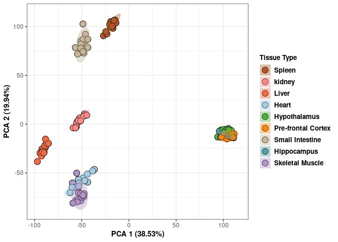
Treatment
Treatment_color <- as.factor(tdata.FPKM.sample.info$Treatment)
Treatment_color <- as.data.frame(Treatment_color)
col_treatment <- colorRampPalette(brewer.pal(n = 12, name = "Paired"))(2)[Treatment_color$Treatment_color]
pca_treatment <- cbind(Treatment_color,pca$x[,1],pca$x[,2])
pca_treatment <- as.data.frame(pca_treatment)

p <- ggplot(pca_treatment,aes(pca$x[,1], pca$x[,2]))
p <- p + geom_point(aes(fill = as.factor(pca_treatment$Treatment_color)), shape=21, size=4) + theme_bw()
p <- p + theme(legend.title = element_text(size=10,face="bold")) +
  theme(legend.text = element_text(size=10, face="bold"))
p <- p + xlab("PCA 1 (38.53%)") + ylab("PCA 2 (19.94%)") + theme(axis.title = element_text(face="bold"))
p <- p + stat_ellipse(aes(pca$x[,1], pca$x[,2], group = Treatment_color, fill = as.factor(pca_treatment$Treatment_color)), geom="polygon",level=0.8,alpha=0.4) +
  scale_fill_manual(values=c("#A6CEE3", "#B15928"),name="Treatment Type",
                       breaks=c("2DG", "None"),
                       labels=c("2DG", "Control")) +
  scale_linetype_manual(values=c(1,2))
print(p)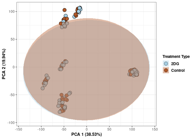
Time
Time_color <- as.factor(tdata.FPKM.sample.info$Time)
Time_color <- as.data.frame(Time_color)
col_time <- colorRampPalette(brewer.pal(n = 12, name = "Paired"))(2)[Time_color$Time_color]
pca_time <- cbind(Time_color,pca$x[,1],pca$x[,2])
pca_time <- as.data.frame(pca_time)

p <- ggplot(pca_time,aes(pca$x[,1], pca$x[,2]))
p <- p + geom_point(aes(fill = as.factor(pca_time$Time_color)), shape=21, size=4) + theme_bw()
p <- p + theme(legend.title = element_text(size=10,face="bold")) +
  theme(legend.text = element_text(size=10, face="bold"))
p <- p + xlab("PCA 1 (38.53%)") + ylab("PCA 2 (19.94%)") + theme(axis.title = element_text(face="bold"))
p <- p + stat_ellipse(aes(pca$x[,1], pca$x[,2], group = Time_color, fill = as.factor(pca_time$Time_color)), geom="polygon",level=0.95,alpha=0.4) +
  scale_fill_manual(values=c("#A6CEE3", "#B15928"),name="Time",
                       breaks=c("4 wks", "96 hrs"),
                       labels=c("4 wks", "96 hrs")) +
  scale_linetype_manual(values=c(1,2))
print(p)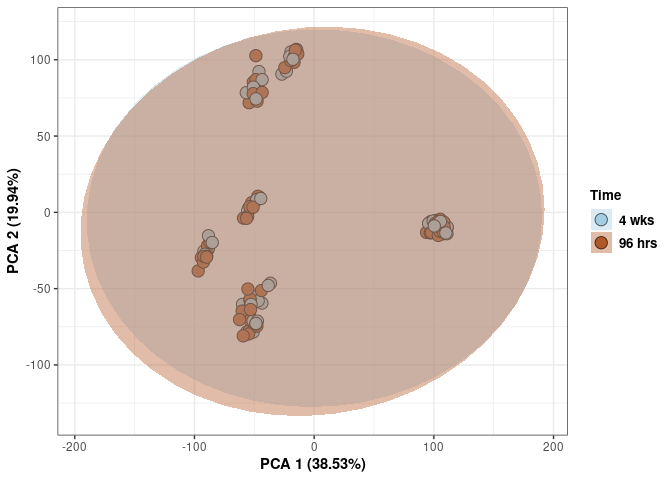
3D PCA
This plot is color coded by tissue, treatment, and time. To see each one click the names on the legend to make them disappear and click again to make them reappear.
Tissue_color <- as.factor(tdata.FPKM.sample.info$Tissue)
Treatment_color <- as.factor(tdata.FPKM.sample.info$Treatment)
Time_color <- as.factor(tdata.FPKM.sample.info$Time)
all_color <- cbind(Tissue_color,Treatment_color,Time_color)
all_color <- as.data.frame(all_color)

col_tissue <- colorRampPalette(brewer.pal(n = 12, name = "Paired"))(9)[all_color$Tissue_color]
col_treatment <- colorRampPalette(brewer.pal(n = 8, name = "Dark2"))(2)[all_color$Treatment_color]
col_time <- colorRampPalette(brewer.pal(n = 12, name = "Set3"))(2)[all_color$Time_color]

pca_all <- cbind(pca$x[,1],pca$x[,2],pca$x[,3],all_color)
pca_all <- as.data.frame(pca_all)
rownames(pca_all) <- rownames(tdata.FPKM.sample.info)

p <- plot_ly(data=pca_all, x = pca_all$`pca$x[, 1]`, y = pca_all$`pca$x[, 2]`, z = pca_all$`pca$x[, 3]`, color = Tissue_color, colors = unique(col_tissue), text = rownames(pca_all)) %>%
  add_markers() %>%
  layout(scene = list(xaxis = list(title = "PC 1 38.53%"),
                     yaxis = list(title = "PC 2 19.94%"),
                     zaxis = list(title = "PC 3 13.47%")))
p1 <- plot_ly(data=pca_all, x = pca_all$`pca$x[, 1]`, y = pca_all$`pca$x[, 2]`, z = pca_all$`pca$x[, 3]`, color = Time_color, colors = unique(col_time), text = rownames(pca_all)) %>%
  add_markers() %>%
  layout(scene = list(xaxis = list(title = "PC 1 38.53%"),
                     yaxis = list(title = "PC 2 19.94%"),
                     zaxis = list(title = "PC 3 13.47%")))

p2 <- plot_ly(data=pca_all, x = pca_all$`pca$x[, 1]`, y = pca_all$`pca$x[, 2]`, z = pca_all$`pca$x[, 3]`, color = Treatment_color, colors = unique(col_treatment), text = rownames(pca_all)) %>%
  add_markers() %>%
  layout(scene = list(xaxis = list(title = "PC 1 38.53%"),
                     yaxis = list(title = "PC 2 19.94%"),
                     zaxis = list(title = "PC 3 13.47%")))

p3 <- plotly::subplot(p,p2,p1)
p3
PCA (log Time)
These plots subset the data so all tissues and treatments are plotted for a single time point.
Scree plot and summary statistics 96 hrs
tdata.FPKM.sample.info <- readRDS(here("Data","20190406_RNAseq_B6_4wk_2DG_counts_phenotypes.RData"))

tdata.FPKM.sample.info.96hr <- rownames_to_column(tdata.FPKM.sample.info) %>% filter(Time=="96 hrs") %>% column_to_rownames('rowname')

tdata.FPKM <- readRDS(here("Data","20190406_RNAseq_B6_4wk_2DG_counts_numeric.RData"))

log.tdata.FPKM <- log(tdata.FPKM + 1)
log.tdata.FPKM <- as.data.frame(log.tdata.FPKM)

rows <- rownames(tdata.FPKM.sample.info.96hr)

log.tdata.FPKM.96hr <- rownames_to_column(log.tdata.FPKM)

log.tdata.FPKM.96hr <- log.tdata.FPKM.96hr %>% filter(rowname %in% rows) %>% column_to_rownames('rowname')

pca <- prcomp(log.tdata.FPKM.96hr, center = T)

screeplot(pca,type = "lines")
summary(pca)## Importance of components:
## PC1 PC2 PC3 PC4 PC5 PC6
## Standard deviation 77.1929 55.9970 45.1005 38.1827 31.37099 20.23438
## Proportion of Variance 0.3907 0.2056 0.1334 0.0956 0.06453 0.02685
## Cumulative Proportion 0.3907 0.5963 0.7297 0.8253 0.88985 0.91669
## PC7 PC8 PC9 PC10 PC11 PC12
## Standard deviation 15.09769 11.55015 11.23114 8.51470 8.11855 6.50039
## Proportion of Variance 0.01495 0.00875 0.00827 0.00475 0.00432 0.00277
## Cumulative Proportion 0.93164 0.94039 0.94866 0.95341 0.95773 0.96051
## PC13 PC14 PC15 PC16 PC17 PC18 PC19
## Standard deviation 5.78054 5.32567 5.07890 5.05911 4.7901 4.50807 4.4443
## Proportion of Variance 0.00219 0.00186 0.00169 0.00168 0.0015 0.00133 0.0013
## Cumulative Proportion 0.96270 0.96456 0.96625 0.96793 0.9694 0.97076 0.9721
## PC20 PC21 PC22 PC23 PC24 PC25 PC26
## Standard deviation 4.31107 4.07696 4.00393 3.84502 3.7009 3.66980 3.59894
## Proportion of Variance 0.00122 0.00109 0.00105 0.00097 0.0009 0.00088 0.00085
## Cumulative Proportion 0.97328 0.97437 0.97542 0.97639 0.9773 0.97817 0.97902
## PC27 PC28 PC29 PC30 PC31 PC32 PC33
## Standard deviation 3.52837 3.46516 3.37063 3.29310 3.2736 3.18494 3.16303
## Proportion of Variance 0.00082 0.00079 0.00074 0.00071 0.0007 0.00067 0.00066
## Cumulative Proportion 0.97983 0.98062 0.98137 0.98208 0.9828 0.98345 0.98410
## PC34 PC35 PC36 PC37 PC38 PC39 PC40
## Standard deviation 3.11314 3.04481 3.00774 2.95572 2.94791 2.88683 2.88075
## Proportion of Variance 0.00064 0.00061 0.00059 0.00057 0.00057 0.00055 0.00054
## Cumulative Proportion 0.98474 0.98535 0.98594 0.98651 0.98708 0.98763 0.98817
## PC41 PC42 PC43 PC44 PC45 PC46 PC47
## Standard deviation 2.81860 2.78743 2.78093 2.71717 2.68201 2.64534 2.63859
## Proportion of Variance 0.00052 0.00051 0.00051 0.00048 0.00047 0.00046 0.00046
## Cumulative Proportion 0.98869 0.98920 0.98971 0.99019 0.99067 0.99112 0.99158
## PC48 PC49 PC50 PC51 PC52 PC53 PC54
## Standard deviation 2.61728 2.57961 2.55437 2.49870 2.49236 2.45412 2.43013
## Proportion of Variance 0.00045 0.00044 0.00043 0.00041 0.00041 0.00039 0.00039
## Cumulative Proportion 0.99203 0.99247 0.99289 0.99330 0.99371 0.99411 0.99449
## PC55 PC56 PC57 PC58 PC59 PC60 PC61
## Standard deviation 2.41504 2.39249 2.36651 2.32658 2.29979 2.27631 2.26294
## Proportion of Variance 0.00038 0.00038 0.00037 0.00035 0.00035 0.00034 0.00034
## Cumulative Proportion 0.99488 0.99525 0.99562 0.99597 0.99632 0.99666 0.99700
## PC62 PC63 PC64 PC65 PC66 PC67 PC68
## Standard deviation 2.25214 2.23049 2.19454 2.15829 2.1437 2.11950 2.11677
## Proportion of Variance 0.00033 0.00033 0.00032 0.00031 0.0003 0.00029 0.00029
## Cumulative Proportion 0.99733 0.99765 0.99797 0.99828 0.9986 0.99887 0.99916
## PC69 PC70 PC71 PC72
## Standard deviation 2.09409 2.08433 2.00131 5.991e-14
## Proportion of Variance 0.00029 0.00028 0.00026 0.000e+00
## Cumulative Proportion 0.99945 0.99974 1.00000 1.000e+00Tissue 96 hrs
Tissue_color <- as.factor(tdata.FPKM.sample.info.96hr$Tissue)
Tissue_color <- as.data.frame(Tissue_color)
col_tissue <- colorRampPalette(brewer.pal(n = 12, name = "Paired"))(9)[Tissue_color$Tissue_color]
pca_tissue <- cbind(Tissue_color,pca$x[,1],pca$x[,2])
pca_tissue <- as.data.frame(pca_tissue)

p <- ggplot(pca_tissue,aes(pca$x[,1], pca$x[,2]))
p <- p + geom_point(aes(fill = as.factor(pca_tissue$Tissue_color)), shape=21, size=4) + theme_bw()
p <- p + theme(legend.title = element_text(size=10,face="bold")) +
  theme(legend.text = element_text(size=10, face="bold"))
p <- p+ xlab("PCA 1 (39.07%)") + ylab("PCA 2 (20.56%)") + theme(axis.title = element_text(face="bold"))
p <- p + stat_ellipse(aes(pca$x[,1], pca$x[,2], group = Tissue_color, fill = as.factor(pca_tissue$Tissue_color)), geom="polygon",level=0.95,alpha=0.2) +
  scale_fill_manual(values=c("#B15928", "#F88A89", "#F06C45", "#A6CEE3", "#52AF43", "#FE870D", "#C7B699", "#569EA4","#B294C7"),name="Tissue Type",
                       breaks=c("Spleen", "Kidney","Liver","Heart","Hypothanamus","Pre-frontal Cortex","Small Intestine","Hippocampus","Skeletal Muscle"),
                       labels=c("Spleen", "kidney","Liver","Heart","Hypothalamus","Pre-frontal Cortex","Small Intestine","Hippocampus","Skeletal Muscle")) +
  scale_linetype_manual(values=c(1,2,1,2,1))
print(p)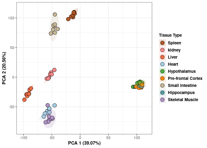
Treatment 96 hrs
Treatment_color <- as.factor(tdata.FPKM.sample.info.96hr$Treatment)
Treatment_color <- as.data.frame(Treatment_color)
col_treatment <- colorRampPalette(brewer.pal(n = 12, name = "Paired"))(2)[Treatment_color$Treatment_color]
pca_treatment <- cbind(Treatment_color,pca$x[,1],pca$x[,2])
pca_treatment <- as.data.frame(pca_treatment)

p <- ggplot(pca_treatment,aes(pca$x[,1], pca$x[,2]))
p <- p + geom_point(aes(fill = as.factor(pca_treatment$Treatment_color)), shape=21, size=4) + theme_bw()
p <- p + theme(legend.title = element_text(size=10,face="bold")) +
  theme(legend.text = element_text(size=10, face="bold"))
p <- p + xlab("PCA 1 (39.07%)") + ylab("PCA 2 (29.56%)") + theme(axis.title = element_text(face="bold"))
p <- p + stat_ellipse(aes(pca$x[,1], pca$x[,2], group = Treatment_color, fill = as.factor(pca_treatment$Treatment_color)), geom="polygon",level=0.95,alpha=0.4) +
  scale_fill_manual(values=c("#A6CEE3", "#B15928"),name="Treatment Type",
                       breaks=c("2DG", "None"),
                       labels=c("2DG", "Control")) +
  scale_linetype_manual(values=c(1,2))
print(p)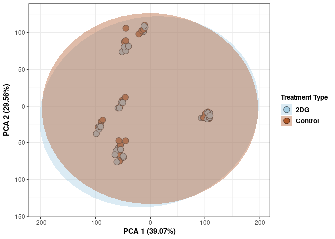
3D Tissue 96 hrs
This plot is color coded by tissue and treatment at 96hrs. To see each one click the names on the legend to make them disappear and click again to make them reappear.
Tissue_color <- as.factor(tdata.FPKM.sample.info.96hr$Tissue)
Tissue_color <- as.data.frame(Tissue_color)
col_tissue <- colorRampPalette(brewer.pal(n = 12, name = "Paired"))(9)[Tissue_color$Tissue_color]
pca_tissue <- cbind(Tissue_color,pca$x[,1],pca$x[,2], pca$x[,3])
pca_tissue <- as.data.frame(pca_tissue)
rownames(pca_tissue) <- rownames(tdata.FPKM.sample.info.96hr)

p <- plot_ly(pca_tissue, x = pca_tissue$`pca$x[, 1]`, y = pca_tissue$`pca$x[, 2]`, z = pca_tissue$`pca$x[, 3]`, color = pca_tissue$Tissue_color, colors = c("#B15928", "#F88A89", "#F06C45", "#A6CEE3", "#52AF43", "#FE870D", "#C7B699", "#569EA4","#B294C7"), text = rownames(pca_tissue)) %>%
  add_markers() %>%
  layout(scene = list(xaxis = list(title = "PC 1 39.07%"),
                     yaxis = list(title = "PC 2 20.56%"),
                     zaxis = list(title = "PC 3 13.34%")))

Treatment_color <- as.factor(tdata.FPKM.sample.info.96hr$Treatment)
Treatment_color <- as.data.frame(Treatment_color)
col_treatment <- colorRampPalette(brewer.pal(n = 12, name = "Paired"))(2)[Treatment_color$Treatment_color]
pca_treatment <- cbind(Treatment_color,pca$x[,1],pca$x[,2],pca$x[,3])
pca_treatment <- as.data.frame(pca_treatment)
rownames(pca_treatment) <- rownames(tdata.FPKM.sample.info.96hr)

p1 <- plot_ly(pca_treatment, x = pca_treatment$`pca$x[, 1]`, y = pca_treatment$`pca$x[, 2]`, z = pca_treatment$`pca$x[, 3]`, color = pca_treatment$Treatment_color, colors = c("#A6CEE3", "#B15928"), text = rownames(pca_treatment)) %>%
  add_markers() %>%
  layout(scene = list(xaxis = list(title = "PC 1 39.07%"),
                     yaxis = list(title = "PC 2 20.56%"),
                     zaxis = list(title = "PC 3 13.34%")))
p2 <-plotly::subplot(p,p1)
p2
Scree plot and summary statistics 4 wks
tdata.FPKM.sample.info <- readRDS(here("Data","20190406_RNAseq_B6_4wk_2DG_counts_phenotypes.RData"))

tdata.FPKM.sample.info.4wk <- rownames_to_column(tdata.FPKM.sample.info) %>% filter(Time=="4 wks") %>% column_to_rownames('rowname')

tdata.FPKM <- readRDS(here("Data","20190406_RNAseq_B6_4wk_2DG_counts_numeric.RData"))

log.tdata.FPKM <- log(tdata.FPKM + 1)
log.tdata.FPKM <- as.data.frame(log.tdata.FPKM)

rows <- rownames(tdata.FPKM.sample.info.4wk)

log.tdata.FPKM.4wk <- rownames_to_column(log.tdata.FPKM)

log.tdata.FPKM.4wk <- log.tdata.FPKM.4wk %>% filter(rowname %in% rows) %>% column_to_rownames('rowname')

pca <- prcomp(log.tdata.FPKM.96hr, center = T)

screeplot(pca,type = "lines")
summary(pca)## Importance of components:
## PC1 PC2 PC3 PC4 PC5 PC6
## Standard deviation 77.1929 55.9970 45.1005 38.1827 31.37099 20.23438
## Proportion of Variance 0.3907 0.2056 0.1334 0.0956 0.06453 0.02685
## Cumulative Proportion 0.3907 0.5963 0.7297 0.8253 0.88985 0.91669
## PC7 PC8 PC9 PC10 PC11 PC12
## Standard deviation 15.09769 11.55015 11.23114 8.51470 8.11855 6.50039
## Proportion of Variance 0.01495 0.00875 0.00827 0.00475 0.00432 0.00277
## Cumulative Proportion 0.93164 0.94039 0.94866 0.95341 0.95773 0.96051
## PC13 PC14 PC15 PC16 PC17 PC18 PC19
## Standard deviation 5.78054 5.32567 5.07890 5.05911 4.7901 4.50807 4.4443
## Proportion of Variance 0.00219 0.00186 0.00169 0.00168 0.0015 0.00133 0.0013
## Cumulative Proportion 0.96270 0.96456 0.96625 0.96793 0.9694 0.97076 0.9721
## PC20 PC21 PC22 PC23 PC24 PC25 PC26
## Standard deviation 4.31107 4.07696 4.00393 3.84502 3.7009 3.66980 3.59894
## Proportion of Variance 0.00122 0.00109 0.00105 0.00097 0.0009 0.00088 0.00085
## Cumulative Proportion 0.97328 0.97437 0.97542 0.97639 0.9773 0.97817 0.97902
## PC27 PC28 PC29 PC30 PC31 PC32 PC33
## Standard deviation 3.52837 3.46516 3.37063 3.29310 3.2736 3.18494 3.16303
## Proportion of Variance 0.00082 0.00079 0.00074 0.00071 0.0007 0.00067 0.00066
## Cumulative Proportion 0.97983 0.98062 0.98137 0.98208 0.9828 0.98345 0.98410
## PC34 PC35 PC36 PC37 PC38 PC39 PC40
## Standard deviation 3.11314 3.04481 3.00774 2.95572 2.94791 2.88683 2.88075
## Proportion of Variance 0.00064 0.00061 0.00059 0.00057 0.00057 0.00055 0.00054
## Cumulative Proportion 0.98474 0.98535 0.98594 0.98651 0.98708 0.98763 0.98817
## PC41 PC42 PC43 PC44 PC45 PC46 PC47
## Standard deviation 2.81860 2.78743 2.78093 2.71717 2.68201 2.64534 2.63859
## Proportion of Variance 0.00052 0.00051 0.00051 0.00048 0.00047 0.00046 0.00046
## Cumulative Proportion 0.98869 0.98920 0.98971 0.99019 0.99067 0.99112 0.99158
## PC48 PC49 PC50 PC51 PC52 PC53 PC54
## Standard deviation 2.61728 2.57961 2.55437 2.49870 2.49236 2.45412 2.43013
## Proportion of Variance 0.00045 0.00044 0.00043 0.00041 0.00041 0.00039 0.00039
## Cumulative Proportion 0.99203 0.99247 0.99289 0.99330 0.99371 0.99411 0.99449
## PC55 PC56 PC57 PC58 PC59 PC60 PC61
## Standard deviation 2.41504 2.39249 2.36651 2.32658 2.29979 2.27631 2.26294
## Proportion of Variance 0.00038 0.00038 0.00037 0.00035 0.00035 0.00034 0.00034
## Cumulative Proportion 0.99488 0.99525 0.99562 0.99597 0.99632 0.99666 0.99700
## PC62 PC63 PC64 PC65 PC66 PC67 PC68
## Standard deviation 2.25214 2.23049 2.19454 2.15829 2.1437 2.11950 2.11677
## Proportion of Variance 0.00033 0.00033 0.00032 0.00031 0.0003 0.00029 0.00029
## Cumulative Proportion 0.99733 0.99765 0.99797 0.99828 0.9986 0.99887 0.99916
## PC69 PC70 PC71 PC72
## Standard deviation 2.09409 2.08433 2.00131 5.991e-14
## Proportion of Variance 0.00029 0.00028 0.00026 0.000e+00
## Cumulative Proportion 0.99945 0.99974 1.00000 1.000e+00Tissue 4 wks
Tissue_color <- as.factor(tdata.FPKM.sample.info.4wk$Tissue)
Tissue_color <- as.data.frame(Tissue_color)
col_tissue <- colorRampPalette(brewer.pal(n = 12, name = "Paired"))(9)[Tissue_color$Tissue_color]
pca_tissue <- cbind(Tissue_color,pca$x[,1],pca$x[,2])
pca_tissue <- as.data.frame(pca_tissue)

p <- ggplot(pca_tissue,aes(pca$x[,1], pca$x[,2]))
p <- p + geom_point(aes(fill = as.factor(pca_tissue$Tissue_color)), shape=21, size=4) + theme_bw()
p <- p + theme(legend.title = element_text(size=10,face="bold")) +
  theme(legend.text = element_text(size=10, face="bold"))
p <- p+ xlab("PCA 1 (39.07%)") + ylab("PCA 2 (20.56%)") + theme(axis.title = element_text(face="bold"))
p <- p + stat_ellipse(aes(pca$x[,1], pca$x[,2], group = Tissue_color, fill = as.factor(pca_tissue$Tissue_color)), geom="polygon",level=0.95,alpha=0.2) +
  scale_fill_manual(values=c("#B15928", "#F88A89", "#F06C45", "#A6CEE3", "#52AF43", "#FE870D", "#C7B699", "#569EA4","#B294C7"),name="Tissue Type",
                       breaks=c("Spleen", "Kidney","Liver","Heart","Hypothanamus","Pre-frontal Cortex","Small Intestine","Hippocampus","Skeletal Muscle"),
                       labels=c("Spleen", "kidney","Liver","Heart","Hypothalamus","Pre-frontal Cortex","Small Intestine","Hippocampus","Skeletal Muscle")) +
  scale_linetype_manual(values=c(1,2,1,2,1))
print(p)
Treatment 4 wks
Treatment_color <- as.factor(tdata.FPKM.sample.info.4wk$Treatment)
Treatment_color <- as.data.frame(Treatment_color)
col_treatment <- colorRampPalette(brewer.pal(n = 12, name = "Paired"))(2)[Treatment_color$Treatment_color]
pca_treatment <- cbind(Treatment_color,pca$x[,1],pca$x[,2])
pca_treatment <- as.data.frame(pca_treatment)

p <- ggplot(pca_treatment,aes(pca$x[,1], pca$x[,2]))
p <- p + geom_point(aes(fill = as.factor(pca_treatment$Treatment_color)), shape=21, size=4) + theme_bw()
p <- p + theme(legend.title = element_text(size=10,face="bold")) +
  theme(legend.text = element_text(size=10, face="bold"))
p <- p + xlab("PCA 1 (39.07%)") + ylab("PCA 2 (20.56%)") + theme(axis.title = element_text(face="bold"))
p <- p + stat_ellipse(aes(pca$x[,1], pca$x[,2], group = Treatment_color, fill = as.factor(pca_treatment$Treatment_color)), geom="polygon",level=0.95,alpha=0.4) +
  scale_fill_manual(values=c("#A6CEE3", "#B15928"),name="Treatment Type",
                       breaks=c("2DG", "None"),
                       labels=c("2DG", "Control")) +
  scale_linetype_manual(values=c(1,2))
print(p)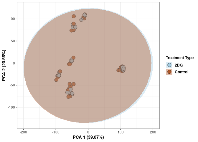
3D 4 wks
This plot is color coded by tissue and treatment at 4wks. To see each one click the names on the legend to make them disappear and click again to make them reappear.
Tissue_color <- as.factor(tdata.FPKM.sample.info.4wk$Tissue)
Tissue_color <- as.data.frame(Tissue_color)
col_tissue <- colorRampPalette(brewer.pal(n = 12, name = "Paired"))(9)[Tissue_color$Tissue_color]
pca_tissue <- cbind(Tissue_color,pca$x[,1],pca$x[,2], pca$x[,3])
pca_tissue <- as.data.frame(pca_tissue)
rownames(pca_tissue) <- rownames(tdata.FPKM.sample.info.4wk)

p <- plot_ly(pca_tissue, x = pca_tissue$`pca$x[, 1]`, y = pca_tissue$`pca$x[, 2]`, z = pca_tissue$`pca$x[, 3]`, color = pca_tissue$Tissue_color, colors = c("#B15928", "#F88A89", "#F06C45", "#A6CEE3", "#52AF43", "#FE870D", "#C7B699", "#569EA4","#B294C7"), text = rownames(pca_tissue)) %>%
  add_markers() %>%
  layout(scene = list(xaxis = list(title = "PC 1 39.07%"),
                     yaxis = list(title = "PC 2 20.56%"),
                     zaxis = list(title = "PC 3 13.34%")))

Treatment_color <- as.factor(tdata.FPKM.sample.info.4wk$Treatment)
Treatment_color <- as.data.frame(Treatment_color)
col_treatment <- colorRampPalette(brewer.pal(n = 12, name = "Paired"))(2)[Treatment_color$Treatment_color]
pca_treatment <- cbind(Treatment_color,pca$x[,1],pca$x[,2],pca$x[,3])
pca_treatment <- as.data.frame(pca_treatment)
rownames(pca_treatment) <- rownames(tdata.FPKM.sample.info.4wk)

p1 <- plot_ly(pca_treatment, x = pca_treatment$`pca$x[, 1]`, y = pca_treatment$`pca$x[, 2]`, z = pca_treatment$`pca$x[, 3]`, color = pca_treatment$Treatment_color, colors = c("#A6CEE3", "#B15928"), text = rownames(pca_treatment)) %>%
  add_markers() %>%
  layout(scene = list(xaxis = list(title = "PC 1 39.07%"),
                     yaxis = list(title = "PC 2 20.56%"),
                     zaxis = list(title = "PC 3 13.34%")))
p2 <-plotly::subplot(p,p1)
p2
PCA (log Treatment)
These plots use subsetted data so the dataset plotted contains all tissues and time points per treatment type (2DG or control).
Scree plot and summary statistics 2DG
tdata.FPKM.sample.info <- readRDS(here("Data","20190406_RNAseq_B6_4wk_2DG_counts_phenotypes.RData"))

tdata.FPKM.sample.info.2DG <- rownames_to_column(tdata.FPKM.sample.info) %>% filter(Treatment=="2DG") %>% column_to_rownames('rowname')

tdata.FPKM <- readRDS(here("Data","20190406_RNAseq_B6_4wk_2DG_counts_numeric.RData"))

log.tdata.FPKM <- log(tdata.FPKM + 1)
log.tdata.FPKM <- as.data.frame(log.tdata.FPKM)

rows <- rownames(tdata.FPKM.sample.info.2DG)

log.tdata.FPKM.2DG <- rownames_to_column(log.tdata.FPKM)

log.tdata.FPKM.2DG <- log.tdata.FPKM.2DG %>% filter(rowname %in% rows) %>% column_to_rownames('rowname')

pca <- prcomp(log.tdata.FPKM.2DG, center = T)

screeplot(pca,type = "lines")
summary(pca)## Importance of components:
## PC1 PC2 PC3 PC4 PC5 PC6
## Standard deviation 76.7746 54.5939 45.2867 38.46225 31.75837 19.70521
## Proportion of Variance 0.3903 0.1974 0.1358 0.09797 0.06679 0.02571
## Cumulative Proportion 0.3903 0.5877 0.7235 0.82150 0.88829 0.91400
## PC7 PC8 PC9 PC10 PC11 PC12
## Standard deviation 14.93515 13.27074 10.59044 8.01944 6.98030 6.73653
## Proportion of Variance 0.01477 0.01166 0.00743 0.00426 0.00323 0.00301
## Cumulative Proportion 0.92878 0.94044 0.94787 0.95212 0.95535 0.95836
## PC13 PC14 PC15 PC16 PC17 PC18 PC19
## Standard deviation 6.27524 5.98189 5.70238 5.15973 4.99381 4.72330 4.50465
## Proportion of Variance 0.00261 0.00237 0.00215 0.00176 0.00165 0.00148 0.00134
## Cumulative Proportion 0.96096 0.96333 0.96549 0.96725 0.96890 0.97038 0.97172
## PC20 PC21 PC22 PC23 PC24 PC25 PC26
## Standard deviation 4.16635 4.13772 3.85635 3.84173 3.75684 3.66018 3.53290
## Proportion of Variance 0.00115 0.00113 0.00098 0.00098 0.00093 0.00089 0.00083
## Cumulative Proportion 0.97287 0.97401 0.97499 0.97597 0.97690 0.97779 0.97862
## PC27 PC28 PC29 PC30 PC31 PC32 PC33
## Standard deviation 3.50511 3.40358 3.27393 3.2560 3.21875 3.17510 3.13050
## Proportion of Variance 0.00081 0.00077 0.00071 0.0007 0.00069 0.00067 0.00065
## Cumulative Proportion 0.97943 0.98020 0.98091 0.9816 0.98230 0.98296 0.98361
## PC34 PC35 PC36 PC37 PC38 PC39 PC40
## Standard deviation 3.08590 3.05920 3.0137 2.98733 2.96858 2.92001 2.87885
## Proportion of Variance 0.00063 0.00062 0.0006 0.00059 0.00058 0.00056 0.00055
## Cumulative Proportion 0.98424 0.98486 0.9855 0.98606 0.98664 0.98720 0.98775
## PC41 PC42 PC43 PC44 PC45 PC46 PC47
## Standard deviation 2.84104 2.81536 2.78572 2.7574 2.73316 2.69189 2.64811
## Proportion of Variance 0.00053 0.00052 0.00051 0.0005 0.00049 0.00048 0.00046
## Cumulative Proportion 0.98829 0.98881 0.98933 0.9898 0.99032 0.99080 0.99127
## PC48 PC49 PC50 PC51 PC52 PC53 PC54
## Standard deviation 2.63257 2.59136 2.56531 2.52373 2.51731 2.49449 2.4720
## Proportion of Variance 0.00046 0.00044 0.00044 0.00042 0.00042 0.00041 0.0004
## Cumulative Proportion 0.99173 0.99217 0.99261 0.99303 0.99345 0.99386 0.9943
## PC55 PC56 PC57 PC58 PC59 PC60 PC61
## Standard deviation 2.4612 2.41862 2.38911 2.37986 2.36155 2.34028 2.27947
## Proportion of Variance 0.0004 0.00039 0.00038 0.00038 0.00037 0.00036 0.00034
## Cumulative Proportion 0.9947 0.99505 0.99543 0.99581 0.99618 0.99654 0.99688
## PC62 PC63 PC64 PC65 PC66 PC67 PC68
## Standard deviation 2.27166 2.24859 2.21900 2.20230 2.19745 2.16513 2.1420
## Proportion of Variance 0.00034 0.00033 0.00033 0.00032 0.00032 0.00031 0.0003
## Cumulative Proportion 0.99723 0.99756 0.99789 0.99821 0.99853 0.99884 0.9991
## PC69 PC70 PC71 PC72
## Standard deviation 2.1133 2.08132 2.04098 3.808e-14
## Proportion of Variance 0.0003 0.00029 0.00028 0.000e+00
## Cumulative Proportion 0.9994 0.99972 1.00000 1.000e+00Tissue 2DG
Tissue_color <- as.factor(tdata.FPKM.sample.info.2DG$Tissue)
Tissue_color <- as.data.frame(Tissue_color)
col_tissue <- colorRampPalette(brewer.pal(n = 12, name = "Paired"))(9)[Tissue_color$Tissue_color]
pca_tissue <- cbind(Tissue_color,pca$x[,1],pca$x[,2])
pca_tissue <- as.data.frame(pca_tissue)

p <- ggplot(pca_tissue,aes(pca$x[,1], pca$x[,2]))
p <- p + geom_point(aes(fill = as.factor(pca_tissue$Tissue_color)), shape=21, size=4) + theme_bw()
p <- p + theme(legend.title = element_text(size=10,face="bold")) +
  theme(legend.text = element_text(size=10, face="bold"))
p <- p+ xlab("PCA 1 (39.03%)") + ylab("PCA 2 (19.74%)") + theme(axis.title = element_text(face="bold"))
p <- p + stat_ellipse(aes(pca$x[,1], pca$x[,2], group = Tissue_color, fill = as.factor(pca_tissue$Tissue_color)), geom="polygon",level=0.95,alpha=0.2) +
  scale_fill_manual(values=c("#B15928", "#F88A89", "#F06C45", "#A6CEE3", "#52AF43", "#FE870D", "#C7B699", "#569EA4","#B294C7"),name="Tissue Type",
                       breaks=c("Spleen", "Kidney","Liver","Heart","Hypothanamus","Pre-frontal Cortex","Small Intestine","Hippocampus","Skeletal Muscle"),
                       labels=c("Spleen", "kidney","Liver","Heart","Hypothalamus","Pre-frontal Cortex","Small Intestine","Hippocampus","Skeletal Muscle")) +
  scale_linetype_manual(values=c(1,2,1,2,1))
print(p)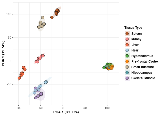
Time 2DG
Time_color <- as.factor(tdata.FPKM.sample.info.2DG$Time)
Time_color <- as.data.frame(Time_color)
col_time <- colorRampPalette(brewer.pal(n = 12, name = "Paired"))(2)[Time_color$Time_color]
pca_time <- cbind(Time_color,pca$x[,1],pca$x[,2])
pca_time <- as.data.frame(pca_time)

p <- ggplot(pca_time,aes(pca$x[,1], pca$x[,2]))
p <- p + geom_point(aes(fill = as.factor(pca_time$Time_color)), shape=21, size=4) + theme_bw()
p <- p + theme(legend.title = element_text(size=10,face="bold")) +
  theme(legend.text = element_text(size=10, face="bold"))
p <- p + xlab("PCA 1 (39.03%)") + ylab("PCA 2 (19.74%)") + theme(axis.title = element_text(face="bold"))
p <- p + stat_ellipse(aes(pca$x[,1], pca$x[,2], group = Time_color, fill = as.factor(pca_time$Time_color)), geom="polygon",level=0.95,alpha=0.4) +
  scale_fill_manual(values=c("#A6CEE3", "#B15928"),name="Time",
                       breaks=c("4 wks", "96 hrs"),
                       labels=c("4 wks", "96 hrs")) +
  scale_linetype_manual(values=c(1,2))
print(p)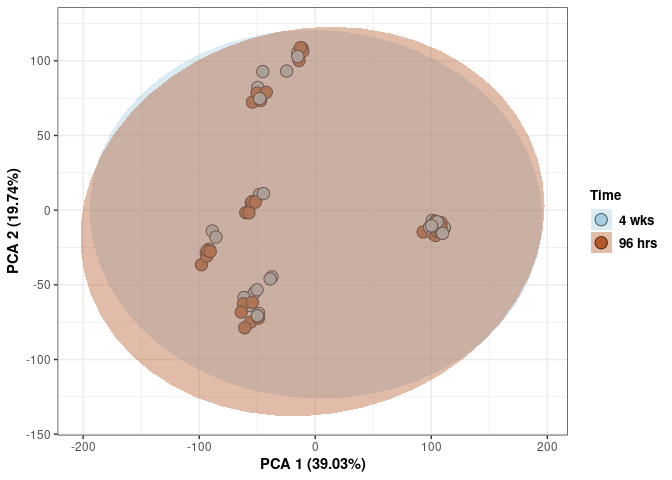
3D Tissue 2DG
This plot is color coded by tissue and time for 2DG. To see each one click the names on the legend to make them disappear and click again to make them reappear.
Tissue_color <- as.factor(tdata.FPKM.sample.info.2DG$Tissue)
Tissue_color <- as.data.frame(Tissue_color)
col_tissue <- colorRampPalette(brewer.pal(n = 12, name = "Paired"))(9)[Tissue_color$Tissue_color]
pca_tissue <- cbind(Tissue_color,pca$x[,1],pca$x[,2],pca$x[,3])
pca_tissue <- as.data.frame(pca_tissue)
rownames(pca_tissue) <- rownames(tdata.FPKM.sample.info.2DG)

p <- plot_ly(pca_tissue, x = pca_tissue$`pca$x[, 1]`, y = pca_tissue$`pca$x[, 2]`, z = pca_tissue$`pca$x[, 3]`, color = pca_tissue$Tissue_color, colors = c("#B15928", "#F88A89", "#F06C45", "#A6CEE3", "#52AF43", "#FE870D", "#C7B699", "#569EA4","#B294C7"), text = rownames(pca_tissue)) %>%
  add_markers() %>%
  layout(scene = list(xaxis = list(title = "PC 1 39.03%"),
                     yaxis = list(title = "PC 2 19.74%"),
                     zaxis = list(title = "PC 3 13.58%")))

Time_color <- as.factor(tdata.FPKM.sample.info.2DG$Time)
Time_color <- as.data.frame(Time_color)
col_time <- colorRampPalette(brewer.pal(n = 12, name = "Paired"))(2)[Time_color$Time_color]
pca_time <- cbind(Time_color,pca$x[,1],pca$x[,2],pca$x[,3])
pca_time <- as.data.frame(pca_time)
rownames(pca_tissue) <- rownames(tdata.FPKM.sample.info.2DG)

p1 <- plot_ly(pca_time, x = pca_time$`pca$x[, 1]`, y = pca_time$`pca$x[, 2]`, z = pca_time$`pca$x[, 3]`, color = pca_time$Time_color, colors = c("#A6CEE3", "#B15928"), text = rownames(pca_time)) %>%
  add_markers() %>%
  layout(scene = list(xaxis = list(title = "PC 1 39.03%"),
                     yaxis = list(title = "PC 2 19.74%"),
                     zaxis = list(title = "PC 3 13.58%")))
p2 <- plotly::subplot(p,p1)
p2
Scree plot and summary statistics control
tdata.FPKM.sample.info <- readRDS(here("Data","20190406_RNAseq_B6_4wk_2DG_counts_phenotypes.RData"))

tdata.FPKM.sample.info.control <- rownames_to_column(tdata.FPKM.sample.info) %>% filter(Treatment=="None") %>% column_to_rownames('rowname')

tdata.FPKM <- readRDS(here("Data","20190406_RNAseq_B6_4wk_2DG_counts_numeric.RData"))

log.tdata.FPKM <- log(tdata.FPKM + 1)
log.tdata.FPKM <- as.data.frame(log.tdata.FPKM)

rows <- rownames(tdata.FPKM.sample.info.control)

log.tdata.FPKM.control <- rownames_to_column(log.tdata.FPKM)

log.tdata.FPKM.control <- log.tdata.FPKM.control %>% filter(rowname %in% rows) %>% column_to_rownames('rowname')

pca <- prcomp(log.tdata.FPKM.control, center = T)

screeplot(pca,type = "lines")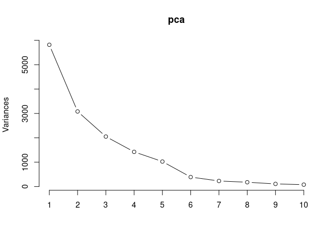
summary(pca)## Importance of components:
## PC1 PC2 PC3 PC4 PC5 PC6
## Standard deviation 76.2724 55.5098 45.2785 37.71954 32.01857 19.72320
## Proportion of Variance 0.3837 0.2033 0.1352 0.09385 0.06763 0.02566
## Cumulative Proportion 0.3837 0.5870 0.7222 0.81610 0.88372 0.90938
## PC7 PC8 PC9 PC10 PC11 PC12
## Standard deviation 15.10005 13.28508 10.39415 8.80560 7.70882 7.4881
## Proportion of Variance 0.01504 0.01164 0.00713 0.00511 0.00392 0.0037
## Cumulative Proportion 0.92442 0.93607 0.94319 0.94831 0.95223 0.9559
## PC13 PC14 PC15 PC16 PC17 PC18 PC19
## Standard deviation 6.69912 6.02094 5.69216 5.24017 5.18524 5.03658 4.91448
## Proportion of Variance 0.00296 0.00239 0.00214 0.00181 0.00177 0.00167 0.00159
## Cumulative Proportion 0.95889 0.96128 0.96342 0.96523 0.96700 0.96867 0.97027
## PC20 PC21 PC22 PC23 PC24 PC25 PC26
## Standard deviation 4.68721 4.48286 4.24205 4.19365 4.06463 3.86965 3.76620
## Proportion of Variance 0.00145 0.00133 0.00119 0.00116 0.00109 0.00099 0.00094
## Cumulative Proportion 0.97172 0.97304 0.97423 0.97539 0.97648 0.97747 0.97840
## PC27 PC28 PC29 PC30 PC31 PC32 PC33
## Standard deviation 3.66418 3.60140 3.50957 3.38166 3.34109 3.28516 3.18542
## Proportion of Variance 0.00089 0.00086 0.00081 0.00075 0.00074 0.00071 0.00067
## Cumulative Proportion 0.97929 0.98014 0.98096 0.98171 0.98245 0.98316 0.98383
## PC34 PC35 PC36 PC37 PC38 PC39 PC40
## Standard deviation 3.11558 3.08555 3.03664 3.0203 2.95433 2.90312 2.88807
## Proportion of Variance 0.00064 0.00063 0.00061 0.0006 0.00058 0.00056 0.00055
## Cumulative Proportion 0.98447 0.98510 0.98570 0.9863 0.98688 0.98744 0.98799
## PC41 PC42 PC43 PC44 PC45 PC46 PC47
## Standard deviation 2.85831 2.81164 2.7601 2.73218 2.70620 2.67497 2.65078
## Proportion of Variance 0.00054 0.00052 0.0005 0.00049 0.00048 0.00047 0.00046
## Cumulative Proportion 0.98853 0.98905 0.9896 0.99004 0.99053 0.99100 0.99146
## PC48 PC49 PC50 PC51 PC52 PC53 PC54
## Standard deviation 2.61854 2.56968 2.56590 2.52814 2.52483 2.48163 2.4710
## Proportion of Variance 0.00045 0.00044 0.00043 0.00042 0.00042 0.00041 0.0004
## Cumulative Proportion 0.99191 0.99235 0.99278 0.99321 0.99363 0.99403 0.9944
## PC55 PC56 PC57 PC58 PC59 PC60 PC61
## Standard deviation 2.43843 2.41625 2.39541 2.37885 2.35179 2.30938 2.29707
## Proportion of Variance 0.00039 0.00039 0.00038 0.00037 0.00036 0.00035 0.00035
## Cumulative Proportion 0.99483 0.99521 0.99559 0.99596 0.99633 0.99668 0.99703
## PC62 PC63 PC64 PC65 PC66 PC67 PC68
## Standard deviation 2.25421 2.23179 2.22381 2.18336 2.1392 2.10807 2.09917
## Proportion of Variance 0.00034 0.00033 0.00033 0.00031 0.0003 0.00029 0.00029
## Cumulative Proportion 0.99736 0.99769 0.99802 0.99833 0.9986 0.99893 0.99922
## PC69 PC70 PC71 PC72
## Standard deviation 2.05043 2.01018 1.89623 5.08e-14
## Proportion of Variance 0.00028 0.00027 0.00024 0.00e+00
## Cumulative Proportion 0.99950 0.99976 1.00000 1.00e+00Tissue control
Tissue_color <- as.factor(tdata.FPKM.sample.info.control$Tissue)
Tissue_color <- as.data.frame(Tissue_color)
col_tissue <- colorRampPalette(brewer.pal(n = 12, name = "Paired"))(9)[Tissue_color$Tissue_color]
pca_tissue <- cbind(Tissue_color,pca$x[,1],pca$x[,2])
pca_tissue <- as.data.frame(pca_tissue)

p <- ggplot(pca_tissue,aes(pca$x[,1], pca$x[,2]))
p <- p + geom_point(aes(fill = as.factor(pca_tissue$Tissue_color)), shape=21, size=4) + theme_bw()
p <- p + theme(legend.title = element_text(size=10,face="bold")) +
  theme(legend.text = element_text(size=10, face="bold"))
p <- p+ xlab("PCA 1 (38.37%)") + ylab("PCA 2 (20.33%)") + theme(axis.title = element_text(face="bold"))
p <- p + stat_ellipse(aes(pca$x[,1], pca$x[,2], group = Tissue_color, fill = as.factor(pca_tissue$Tissue_color)), geom="polygon",level=0.95,alpha=0.2) +
  scale_fill_manual(values=c("#B15928", "#F88A89", "#F06C45", "#A6CEE3", "#52AF43", "#FE870D", "#C7B699", "#569EA4","#B294C7"),name="Tissue Type",
                       breaks=c("Spleen", "Kidney","Liver","Heart","Hypothanamus","Pre-frontal Cortex","Small Intestine","Hippocampus","Skeletal Muscle"),
                       labels=c("Spleen", "kidney","Liver","Heart","Hypothalamus","Pre-frontal Cortex","Small Intestine","Hippocampus","Skeletal Muscle")) +
  scale_linetype_manual(values=c(1,2,1,2,1))
print(p)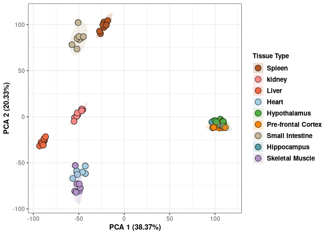
Time control
Time_color <- as.factor(tdata.FPKM.sample.info.control$Time)
Time_color <- as.data.frame(Time_color)
col_time <- colorRampPalette(brewer.pal(n = 12, name = "Paired"))(2)[Time_color$Time_color]
pca_time <- cbind(Time_color,pca$x[,1],pca$x[,2])
pca_time <- as.data.frame(pca_time)

p <- ggplot(pca_time,aes(pca$x[,1], pca$x[,2]))
p <- p + geom_point(aes(fill = as.factor(pca_time$Time_color)), shape=21, size=4) + theme_bw()
p <- p + theme(legend.title = element_text(size=10,face="bold")) +
  theme(legend.text = element_text(size=10, face="bold"))
p <- p + xlab("PCA 1 (38.37%)") + ylab("PCA 2 (20.33%)") + theme(axis.title = element_text(face="bold"))
p <- p + stat_ellipse(aes(pca$x[,1], pca$x[,2], group = Time_color, fill = as.factor(pca_time$Time_color)), geom="polygon",level=0.95,alpha=0.4) +
  scale_fill_manual(values=c("#A6CEE3", "#B15928"),name="Time",
                       breaks=c("4 wks", "96 hrs"),
                       labels=c("4 wks", "96 hrs")) +
  scale_linetype_manual(values=c(1,2))
print(p)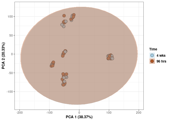
3D Tissue control
This plot is color coded by tissue and time for control. To see each one click the names on the legend to make them disappear and click again to make them reappear.
Tissue_color <- as.factor(tdata.FPKM.sample.info.control$Tissue)
Tissue_color <- as.data.frame(Tissue_color)
col_tissue <- colorRampPalette(brewer.pal(n = 12, name = "Paired"))(9)[Tissue_color$Tissue_color]
pca_tissue <- cbind(Tissue_color,pca$x[,1],pca$x[,2],pca$x[,3])
pca_tissue <- as.data.frame(pca_tissue)
rownames(pca_tissue) <- rownames(tdata.FPKM.sample.info.control)

p <- plot_ly(pca_tissue, x = pca_tissue$`pca$x[, 1]`, y = pca_tissue$`pca$x[, 2]`, z = pca_tissue$`pca$x[, 3]`, color = pca_tissue$Tissue_color, colors = c("#B15928", "#F88A89", "#F06C45", "#A6CEE3", "#52AF43", "#FE870D", "#C7B699", "#569EA4","#B294C7"), text = rownames(pca_tissue)) %>%
  add_markers() %>%
  layout(scene = list(xaxis = list(title = "PC 1 38.37%"),
                     yaxis = list(title = "PC 2 20.33%"),
                     zaxis = list(title = "PC 3 13.52%")))

Time_color <- as.factor(tdata.FPKM.sample.info.control$Time)
Time_color <- as.data.frame(Time_color)
col_time <- colorRampPalette(brewer.pal(n = 12, name = "Paired"))(2)[Time_color$Time_color]
pca_time <- cbind(Time_color,pca$x[,1],pca$x[,2],pca$x[,3])
pca_time <- as.data.frame(pca_time)
rownames(pca_tissue) <- rownames(tdata.FPKM.sample.info.control)

p1 <- plot_ly(pca_time, x = pca_time$`pca$x[, 1]`, y = pca_time$`pca$x[, 2]`, z = pca_time$`pca$x[, 3]`, color = pca_time$Time_color, colors = c("#A6CEE3", "#B15928") , text = rownames(pca_time)) %>%
  add_markers() %>%
  layout(scene = list(xaxis = list(title = "PC 1 38.37%"),
                     yaxis = list(title = "PC 2 20.33%"),
                     zaxis = list(title = "PC 3 13.52%")))
p2 <- plotly::subplot(p,p1)
p2
PCA (log Tissue)
These plots subset the data so each plot contains treatment and time for each tissue.
Scree plot and summary statistics spleen
tdata.FPKM.sample.info <- readRDS(here("Data","20190406_RNAseq_B6_4wk_2DG_counts_phenotypes.RData"))

tdata.FPKM.sample.info.spleen <- rownames_to_column(tdata.FPKM.sample.info) %>% filter(Tissue=="Spleen") %>% column_to_rownames('rowname')

tdata.FPKM <- readRDS(here("Data","20190406_RNAseq_B6_4wk_2DG_counts_numeric.RData"))

log.tdata.FPKM <- log(tdata.FPKM + 1)
log.tdata.FPKM <- as.data.frame(log.tdata.FPKM)

rows <- rownames(tdata.FPKM.sample.info.spleen)

log.tdata.FPKM.spleen <- rownames_to_column(log.tdata.FPKM)

log.tdata.FPKM.spleen <- log.tdata.FPKM.spleen %>% filter(rowname %in% rows) %>% column_to_rownames('rowname')

pca <- prcomp(log.tdata.FPKM.spleen, center = T)

screeplot(pca,type = "lines")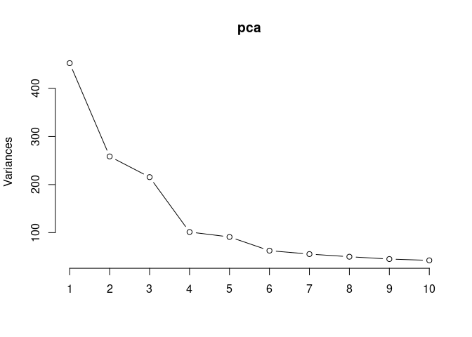
summary(pca)## Importance of components:
## PC1 PC2 PC3 PC4 PC5 PC6 PC7
## Standard deviation 21.2720 16.0785 14.6800 10.06728 9.54473 7.91133 7.44641
## Proportion of Variance 0.2934 0.1676 0.1397 0.06572 0.05907 0.04058 0.03595
## Cumulative Proportion 0.2934 0.4610 0.6008 0.66647 0.72554 0.76612 0.80207
## PC8 PC9 PC10 PC11 PC12 PC13 PC14
## Standard deviation 7.06778 6.71785 6.51051 6.14619 6.07888 5.76171 5.5536
## Proportion of Variance 0.03239 0.02926 0.02748 0.02449 0.02396 0.02152 0.0200
## Cumulative Proportion 0.83446 0.86372 0.89121 0.91570 0.93966 0.96119 0.9812
## PC15 PC16
## Standard deviation 5.38704 1.686e-14
## Proportion of Variance 0.01882 0.000e+00
## Cumulative Proportion 1.00000 1.000e+00Time and treatment spleen
tdata.FPKM.sample.info <- readRDS(here("Data","20190406_RNAseq_B6_4wk_2DG_counts_phenotypes.RData"))

treatment_time <-paste(tdata.FPKM.sample.info$Treatment, tdata.FPKM.sample.info$Time)

tdata.FPKM.sample.info <-cbind(tdata.FPKM.sample.info,treatment_time)

tdata.FPKM.sample.info.spleen <- rownames_to_column(tdata.FPKM.sample.info) %>% filter(Tissue=="Spleen") %>% column_to_rownames('rowname')

tdata.FPKM <- readRDS(here("Data","20190406_RNAseq_B6_4wk_2DG_counts_numeric.RData"))

log.tdata.FPKM <- log(tdata.FPKM + 1)
log.tdata.FPKM <- as.data.frame(log.tdata.FPKM)

rows <- rownames(tdata.FPKM.sample.info.spleen)

log.tdata.FPKM.spleen <- rownames_to_column(log.tdata.FPKM)

log.tdata.FPKM.spleen <- log.tdata.FPKM.spleen %>% filter(rowname %in% rows) %>% column_to_rownames('rowname')

pca <- prcomp(log.tdata.FPKM.spleen, center = T)

screeplot(pca,type = "lines")
summary(pca)## Importance of components:
## PC1 PC2 PC3 PC4 PC5 PC6 PC7
## Standard deviation 21.2720 16.0785 14.6800 10.06728 9.54473 7.91133 7.44641
## Proportion of Variance 0.2934 0.1676 0.1397 0.06572 0.05907 0.04058 0.03595
## Cumulative Proportion 0.2934 0.4610 0.6008 0.66647 0.72554 0.76612 0.80207
## PC8 PC9 PC10 PC11 PC12 PC13 PC14
## Standard deviation 7.06778 6.71785 6.51051 6.14619 6.07888 5.76171 5.5536
## Proportion of Variance 0.03239 0.02926 0.02748 0.02449 0.02396 0.02152 0.0200
## Cumulative Proportion 0.83446 0.86372 0.89121 0.91570 0.93966 0.96119 0.9812
## PC15 PC16
## Standard deviation 5.38704 1.686e-14
## Proportion of Variance 0.01882 0.000e+00
## Cumulative Proportion 1.00000 1.000e+00Treatment_time_color <- as.factor(tdata.FPKM.sample.info.spleen$treatment_time)
Treatment_time_color <- as.data.frame(Treatment_time_color)
col_treatment_time <- colorRampPalette(brewer.pal(n = 12, name = "Paired"))(4)[Treatment_time_color$Treatment_time_color]
pca_treatment_time <- cbind(Treatment_time_color,pca$x[,1],pca$x[,2])
pca_treatment_time <- as.data.frame(pca_treatment_time)
p <- ggplot(pca_treatment_time,aes(pca$x[,1], pca$x[,2]))
p <- p + geom_point(aes(fill = as.factor(pca_treatment_time$Treatment_time_color)), shape=21, size=4) + theme_bw()
p <- p + theme(legend.title = element_text(size=10,face="bold")) +
theme(legend.text = element_text(size=10, face="bold"))
p <- p + xlab("PCA 1 (29.34%)") + ylab("PCA 2 (16.76%)") + theme(axis.title = element_text(face="bold"))
p <- p + stat_ellipse(aes(pca$x[,1], pca$x[,2], group = Treatment_time_color, fill = as.factor(pca_treatment_time$Treatment_time_color)), geom="polygon",level=0.95,alpha=0.4) +
scale_fill_manual(values=c("#ED8F47", "#B89B74", "#A6CEE3", "#B15928"),name="Treatment Type and Time",
breaks=c("None 4 wks", "2DG 96 hrs", "2DG 4 wks", "None 96 hrs"),
labels=c("None 4 wks", "2DG 96 hrs", "2DG 4 wks", "None 96 hrs")) +
scale_linetype_manual(values=c(1,2))
print(p)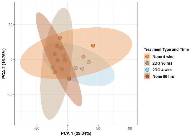
Treatment spleen
Treatment_color <- as.factor(tdata.FPKM.sample.info.spleen$Treatment)
Treatment_color <- as.data.frame(Treatment_color)
col_treatment <- colorRampPalette(brewer.pal(n = 12, name = "Paired"))(2)[Treatment_color$Treatment_color]
pca_treatment <- cbind(Treatment_color,pca$x[,1],pca$x[,2])
pca_treatment <- as.data.frame(pca_treatment)

p <- ggplot(pca_treatment,aes(pca$x[,1], pca$x[,2]))
p <- p + geom_point(aes(fill = as.factor(pca_treatment$Treatment_color)), shape=21, size=4) + theme_bw()
p <- p + theme(legend.title = element_text(size=10,face="bold")) +
  theme(legend.text = element_text(size=10, face="bold"))
p <- p + xlab("PCA 1 (29.34%)") + ylab("PCA 2 (16.76%)") + theme(axis.title = element_text(face="bold"))
p <- p + stat_ellipse(aes(pca$x[,1], pca$x[,2], group = Treatment_color, fill = as.factor(pca_treatment$Treatment_color)), geom="polygon",level=0.95,alpha=0.4) +
  scale_fill_manual(values=c("#A6CEE3", "#B15928"),name="Treatment Type",
                       breaks=c("2DG", "None"),
                       labels=c("2DG", "None")) +
  scale_linetype_manual(values=c(1,2))
print(p)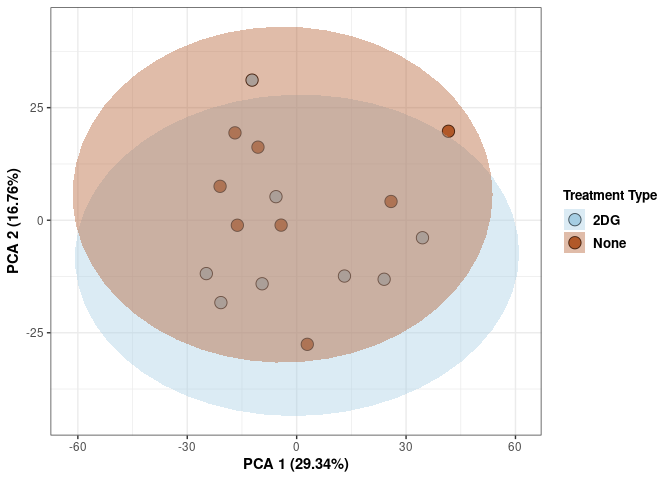
Time spleen
Time_color <- as.factor(tdata.FPKM.sample.info.spleen$Time)
Time_color <- as.data.frame(Time_color)
col_time <- colorRampPalette(brewer.pal(n = 12, name = "Paired"))(2)[Time_color$Time_color]
pca_time <- cbind(Time_color,pca$x[,1],pca$x[,2])
pca_time <- as.data.frame(pca_time)

p <- ggplot(pca_time,aes(pca$x[,1], pca$x[,2]))
p <- p + geom_point(aes(fill = as.factor(pca_time$Time_color)), shape=21, size=4) + theme_bw()
p <- p + theme(legend.title = element_text(size=10,face="bold")) +
  theme(legend.text = element_text(size=10, face="bold"))
p <- p + xlab("PCA 1 (29.34%)") + ylab("PCA 2 (16.76%)") + theme(axis.title = element_text(face="bold"))
p <- p + stat_ellipse(aes(pca$x[,1], pca$x[,2], group = Time_color, fill = as.factor(pca_time$Time_color)), geom="polygon",level=0.95,alpha=0.4) +
  scale_fill_manual(values=c("#A6CEE3", "#B15928"),name="Time",
                       breaks=c("4 wks", "96 hrs"),
                       labels=c("4 wks", "96 hrs")) +
  scale_linetype_manual(values=c(1,2))
print(p)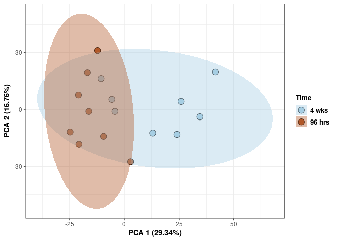
3D spleen
This plot is color coded by time and treatment for spleen, first collectively and then separately. To see each one click the names on the legend to make them disappear and click again to make them reappear.
Treatment_time_color <- as.factor(tdata.FPKM.sample.info.spleen$treatment_time)
Treatment_time_color <- as.data.frame(Treatment_time_color)
col_treatment_time <- colorRampPalette(brewer.pal(n = 12, name = "Paired"))(4)[Treatment_time_color$Treatment_time_color]
pca_treatment_time <- cbind(Treatment_time_color,pca$x[,1],pca$x[,2],pca$x[,3])
pca_treatment_time <- as.data.frame(pca_treatment_time)
rownames(pca_treatment_time) <- rownames(tdata.FPKM.sample.info.spleen)


p <- plot_ly(pca_treatment_time, x = pca_treatment_time$`pca$x[, 1]`, y = pca_treatment_time$`pca$x[, 2]`, z = pca_treatment_time$`pca$x[, 3]`, color = pca_treatment_time$Treatment_time_color, colors = c("#ED8F47", "#B89B74", "#A6CEE3", "#B15928"), text = rownames(pca_treatment_time)) %>%
  add_markers() %>%
  layout(scene = list(xaxis = list(title = "PC 1 29.34%"),
                     yaxis = list(title = "PC 2 16.76%"),
                     zaxis = list(title = "PC 3 13.97%")))

Treatment_color <- as.factor(tdata.FPKM.sample.info.spleen$Treatment)
Treatment_color <- as.data.frame(Treatment_color)
col_treatment <- colorRampPalette(brewer.pal(n = 12, name = "Paired"))(2)[Treatment_color$Treatment_color]
pca_treatment <- cbind(Treatment_color,pca$x[,1],pca$x[,2],pca$x[,3])
pca_treatment <- as.data.frame(pca_treatment)
rownames(pca_treatment) <- rownames(tdata.FPKM.sample.info.spleen)


p1 <- plot_ly(pca_treatment, x = pca_treatment$`pca$x[, 1]`, y = pca_treatment$`pca$x[, 2]`, z = pca_treatment$`pca$x[, 3]`, color = pca_treatment$Treatment_color, colors = c("#CC0000", "#330033"), text = rownames(pca_treatment)) %>%
  add_markers() %>%
  layout(scene = list(xaxis = list(title = "PC 1 29.34%"),
                     yaxis = list(title = "PC 2 16.76%"),
                     zaxis = list(title = "PC 3 13.97%")))

Time_color <- as.factor(tdata.FPKM.sample.info.spleen$Time)
Time_color <- as.data.frame(Time_color)
col_time <- colorRampPalette(brewer.pal(n = 12, name = "Paired"))(2)[Time_color$Time_color]
pca_time <- cbind(Time_color,pca$x[,1],pca$x[,2],pca$x[,3])
pca_time <- as.data.frame(pca_time)
rownames(pca_time) <- rownames(tdata.FPKM.sample.info.spleen)

p2 <- plot_ly(pca_time, x = pca_time$`pca$x[, 1]`, y = pca_time$`pca$x[, 2]`, z = pca_time$`pca$x[, 3]`, color = pca_time$Time_color, colors = c("#B8860B", "#00FA9A"), text = rownames(pca_time)) %>%
  add_markers() %>%
  layout(scene = list(xaxis = list(title = "PC 1 29.34%"),
                     yaxis = list(title = "PC 2 16.76%"),
                     zaxis = list(title = "PC 3 13.97%")))
p3 <- plotly::subplot(p,p1,p2)
p3
Scree plot and summary statistics kidney
tdata.FPKM.sample.info <- readRDS(here("Data","20190406_RNAseq_B6_4wk_2DG_counts_phenotypes.RData"))

tdata.FPKM.sample.info.kidney <- rownames_to_column(tdata.FPKM.sample.info) %>% filter(Tissue=="Kidney") %>% column_to_rownames('rowname')

tdata.FPKM <- readRDS(here("Data","20190406_RNAseq_B6_4wk_2DG_counts_numeric.RData"))

log.tdata.FPKM <- log(tdata.FPKM + 1)
log.tdata.FPKM <- as.data.frame(log.tdata.FPKM)

rows <- rownames(tdata.FPKM.sample.info.kidney)

log.tdata.FPKM.kidney <- rownames_to_column(log.tdata.FPKM)

log.tdata.FPKM.kidney <- log.tdata.FPKM.kidney %>% filter(rowname %in% rows) %>% column_to_rownames('rowname')

pca <- prcomp(log.tdata.FPKM.kidney, center = T)

screeplot(pca,type = "lines")
summary(pca)## Importance of components:
## PC1 PC2 PC3 PC4 PC5 PC6 PC7
## Standard deviation 16.6238 10.5629 9.0495 7.33813 6.79463 6.28965 6.2248
## Proportion of Variance 0.3209 0.1296 0.0951 0.06253 0.05361 0.04594 0.0450
## Cumulative Proportion 0.3209 0.4505 0.5456 0.60811 0.66172 0.70765 0.7527
## PC8 PC9 PC10 PC11 PC12 PC13 PC14
## Standard deviation 5.8546 5.59029 5.36416 5.24261 5.18485 4.89210 4.59934
## Proportion of Variance 0.0398 0.03629 0.03341 0.03192 0.03122 0.02779 0.02456
## Cumulative Proportion 0.7924 0.82874 0.86216 0.89407 0.92529 0.95308 0.97765
## PC15 PC16
## Standard deviation 4.38723 1.491e-14
## Proportion of Variance 0.02235 0.000e+00
## Cumulative Proportion 1.00000 1.000e+00Treatment and time kidney
tdata.FPKM.sample.info <- readRDS(here("Data","20190406_RNAseq_B6_4wk_2DG_counts_phenotypes.RData"))

treatment_time <-paste(tdata.FPKM.sample.info$Treatment, tdata.FPKM.sample.info$Time)

tdata.FPKM.sample.info <-cbind(tdata.FPKM.sample.info,treatment_time)

tdata.FPKM.sample.info.kidney <- rownames_to_column(tdata.FPKM.sample.info) %>% filter(Tissue=="Kidney") %>% column_to_rownames('rowname')

tdata.FPKM <- readRDS(here("Data","20190406_RNAseq_B6_4wk_2DG_counts_numeric.RData"))

log.tdata.FPKM <- log(tdata.FPKM + 1)
log.tdata.FPKM <- as.data.frame(log.tdata.FPKM)

rows <- rownames(tdata.FPKM.sample.info.kidney)

log.tdata.FPKM.kidney <- rownames_to_column(log.tdata.FPKM)

log.tdata.FPKM.kidney <- log.tdata.FPKM.kidney %>% filter(rowname %in% rows) %>% column_to_rownames('rowname')

pca <- prcomp(log.tdata.FPKM.kidney, center = T)

screeplot(pca,type = "lines")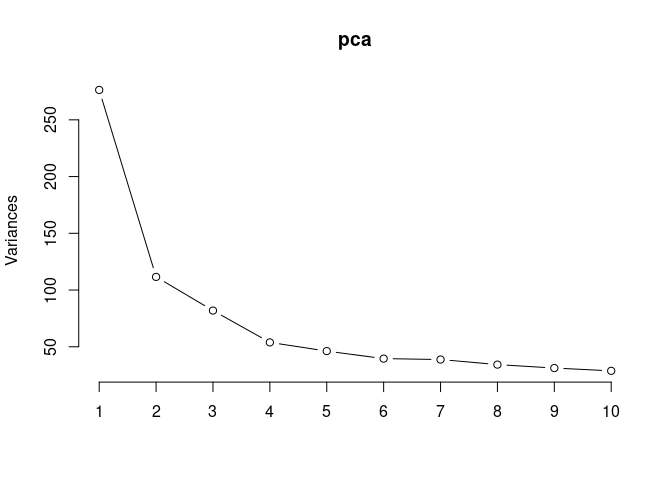
summary(pca)## Importance of components:
## PC1 PC2 PC3 PC4 PC5 PC6 PC7
## Standard deviation 16.6238 10.5629 9.0495 7.33813 6.79463 6.28965 6.2248
## Proportion of Variance 0.3209 0.1296 0.0951 0.06253 0.05361 0.04594 0.0450
## Cumulative Proportion 0.3209 0.4505 0.5456 0.60811 0.66172 0.70765 0.7527
## PC8 PC9 PC10 PC11 PC12 PC13 PC14
## Standard deviation 5.8546 5.59029 5.36416 5.24261 5.18485 4.89210 4.59934
## Proportion of Variance 0.0398 0.03629 0.03341 0.03192 0.03122 0.02779 0.02456
## Cumulative Proportion 0.7924 0.82874 0.86216 0.89407 0.92529 0.95308 0.97765
## PC15 PC16
## Standard deviation 4.38723 1.491e-14
## Proportion of Variance 0.02235 0.000e+00
## Cumulative Proportion 1.00000 1.000e+00Treatment_time_color <- as.factor(tdata.FPKM.sample.info.kidney$treatment_time)
Treatment_time_color <- as.data.frame(Treatment_time_color)
col_treatment_time <- colorRampPalette(brewer.pal(n = 12, name = "Paired"))(4)[Treatment_time_color$Treatment_time_color]
pca_treatment_time <- cbind(Treatment_time_color,pca$x[,1],pca$x[,2])
pca_treatment_time <- as.data.frame(pca_treatment_time)
p <- ggplot(pca_treatment_time,aes(pca$x[,1], pca$x[,2]))
p <- p + geom_point(aes(fill = as.factor(pca_treatment_time$Treatment_time_color)), shape=21, size=4) + theme_bw()
p <- p + theme(legend.title = element_text(size=10,face="bold")) +
theme(legend.text = element_text(size=10, face="bold"))
p <- p + xlab("PCA 1 (32.09%)") + ylab("PCA 2 (12.96%)") + theme(axis.title = element_text(face="bold"))
p <- p + stat_ellipse(aes(pca$x[,1], pca$x[,2], group = Treatment_time_color, fill = as.factor(pca_treatment_time$Treatment_time_color)), geom="polygon",level=0.95,alpha=0.4) +
scale_fill_manual(values=c("#ED8F47", "#B89B74", "#A6CEE3", "#B15928"),name="Treatment Type and Time",
breaks=c("None 4 wks", "2DG 96 hrs", "2DG 4 wks", "None 96 hrs"),
labels=c("None 4 wks", "2DG 96 hrs", "2DG 4 wks", "None 96 hrs")) +
scale_linetype_manual(values=c(1,2))
print(p)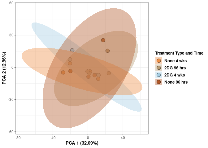
Treatment kidney
Treatment_color <- as.factor(tdata.FPKM.sample.info.kidney$Treatment)
Treatment_color <- as.data.frame(Treatment_color)
col_treatment <- colorRampPalette(brewer.pal(n = 12, name = "Paired"))(2)[Treatment_color$Treatment_color]
pca_treatment <- cbind(Treatment_color,pca$x[,1],pca$x[,2])
pca_treatment <- as.data.frame(pca_treatment)

p <- ggplot(pca_treatment,aes(pca$x[,1], pca$x[,2]))
p <- p + geom_point(aes(fill = as.factor(pca_treatment$Treatment_color)), shape=21, size=4) + theme_bw()
p <- p + theme(legend.title = element_text(size=10,face="bold")) +
  theme(legend.text = element_text(size=10, face="bold"))
p <- p + xlab("PCA 1 (32.09%)") + ylab("PCA 2 (12.96%)") + theme(axis.title = element_text(face="bold"))
p <- p + stat_ellipse(aes(pca$x[,1], pca$x[,2], group = Treatment_color, fill = as.factor(pca_treatment$Treatment_color)), geom="polygon",level=0.95,alpha=0.4) +
  scale_fill_manual(values=c("#A6CEE3", "#B15928"),name="Treatment Type",
                       breaks=c("2DG", "None"),
                       labels=c("2DG", "None")) +
  scale_linetype_manual(values=c(1,2))
print(p)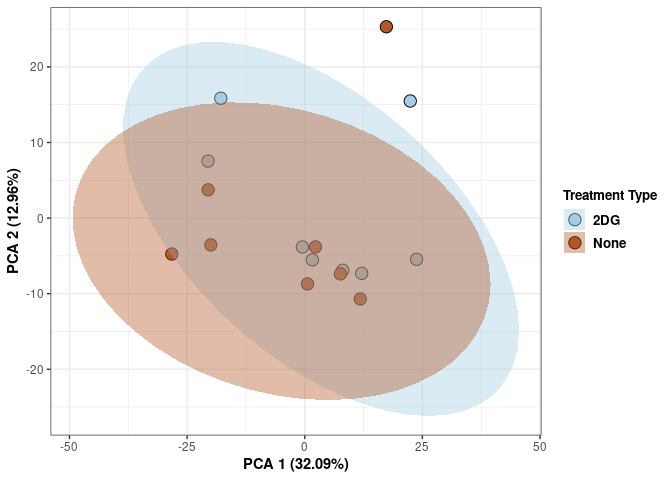
Time kidney
Time_color <- as.factor(tdata.FPKM.sample.info.kidney$Time)
Time_color <- as.data.frame(Time_color)
col_time <- colorRampPalette(brewer.pal(n = 12, name = "Paired"))(2)[Time_color$Time_color]
pca_time <- cbind(Time_color,pca$x[,1],pca$x[,2])
pca_time <- as.data.frame(pca_time)

p <- ggplot(pca_time,aes(pca$x[,1], pca$x[,2]))
p <- p + geom_point(aes(fill = as.factor(pca_time$Time_color)), shape=21, size=4) + theme_bw()
p <- p + theme(legend.title = element_text(size=10,face="bold")) +
  theme(legend.text = element_text(size=10, face="bold"))
p <- p + xlab("PCA 1 (38.53%)") + ylab("PCA 2 (19.94%)") + theme(axis.title = element_text(face="bold"))
p <- p + stat_ellipse(aes(pca$x[,1], pca$x[,2], group = Time_color, fill = as.factor(pca_time$Time_color)), geom="polygon",level=0.95,alpha=0.4) +
  scale_fill_manual(values=c("#A6CEE3", "#B15928"),name="Time",
                       breaks=c("4 wks", "96 hrs"),
                       labels=c("4 wks", "96 hrs")) +
  scale_linetype_manual(values=c(1,2))
print(p)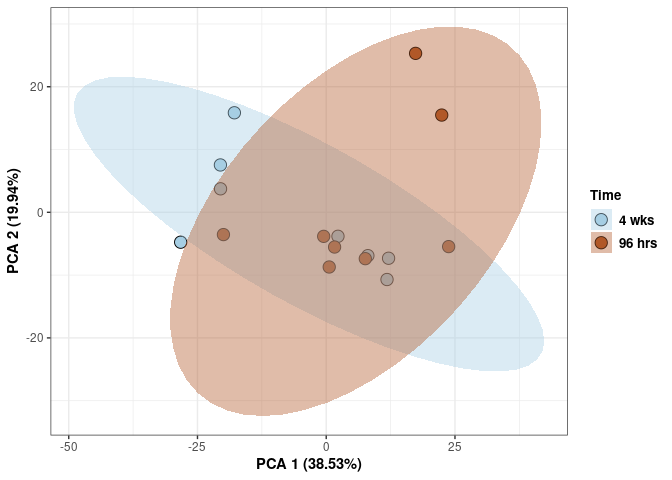
3D kidney
This plot is color coded by time and treatment for kidney, first collectively and then separately. To see each one click the names on the legend to make them disappear and click again to make them reappear.
Treatment_time_color <- as.factor(tdata.FPKM.sample.info.kidney$treatment_time)
Treatment_time_color <- as.data.frame(Treatment_time_color)
col_treatment_time <- colorRampPalette(brewer.pal(n = 12, name = "Paired"))(4)[Treatment_time_color$Treatment_time_color]
pca_treatment_time <- cbind(Treatment_time_color,pca$x[,1],pca$x[,2],pca$x[,3])
pca_treatment_time <- as.data.frame(pca_treatment_time)
rownames(pca_treatment_time) <- rownames(tdata.FPKM.sample.info.kidney)

p <- plot_ly(pca_treatment_time, x = pca_treatment_time$`pca$x[, 1]`, y = pca_treatment_time$`pca$x[, 2]`, z = pca_treatment_time$`pca$x[, 3]`, color = pca_treatment_time$Treatment_time_color, colors = c("#ED8F47", "#B89B74", "#A6CEE3", "#B15928"), text = rownames(pca_treatment_time)) %>%
  add_markers() %>%
  layout(scene = list(xaxis = list(title = "PC 1 32.09%"),
                     yaxis = list(title = "PC 2 12.96%"),
                     zaxis = list(title = "PC 3 9.51%")))

Treatment_color <- as.factor(tdata.FPKM.sample.info.kidney$Treatment)
Treatment_color <- as.data.frame(Treatment_color)
col_treatment <- colorRampPalette(brewer.pal(n = 12, name = "Paired"))(2)[Treatment_color$Treatment_color]
pca_treatment <- cbind(Treatment_color,pca$x[,1],pca$x[,2],pca$x[,3])
pca_treatment <- as.data.frame(pca_treatment)
rownames(pca_treatment) <- rownames(tdata.FPKM.sample.info.kidney)

p1 <- plot_ly(pca_treatment, x = pca_treatment$`pca$x[, 1]`, y = pca_treatment$`pca$x[, 2]`, z = pca_treatment$`pca$x[, 3]`, color = pca_treatment$Treatment_color, colors = c("#CC0000", "#330033"), text = rownames(pca_treatment)) %>%
  add_markers() %>%
  layout(scene = list(xaxis = list(title = "PC 1 32.09%"),
                     yaxis = list(title = "PC 2 12.96%"),
                     zaxis = list(title = "PC 3 9.51%")))

Time_color <- as.factor(tdata.FPKM.sample.info.kidney$Time)
Time_color <- as.data.frame(Time_color)
col_time <- colorRampPalette(brewer.pal(n = 12, name = "Paired"))(2)[Time_color$Time_color]
pca_time <- cbind(Time_color,pca$x[,1],pca$x[,2], pca$x[,3])
pca_time <- as.data.frame(pca_time)
rownames(pca_time) <- rownames(tdata.FPKM.sample.info.kidney)

p2 <- plot_ly(pca_time, x = pca_time$`pca$x[, 1]`, y = pca_time$`pca$x[, 2]`, z = pca_time$`pca$x[, 3]`, color = pca_time$Time_color, colors = c("#B8860B", "#00FA9A"), text = rownames(pca_time)) %>%
  add_markers() %>%
  layout(scene = list(xaxis = list(title = "PC 1 32.09%"),
                     yaxis = list(title = "PC 2 12.96%"),
                     zaxis = list(title = "PC 3 9.51%")))
p3 <- plotly::subplot(p,p1,p2)
p3
Scree plot and summary statistics hypothalamus
tdata.FPKM.sample.info <- readRDS(here("Data","20190406_RNAseq_B6_4wk_2DG_counts_phenotypes.RData"))

tdata.FPKM.sample.info.hypothalamus <- rownames_to_column(tdata.FPKM.sample.info) %>% filter(Tissue=="Hypothanamus") %>% column_to_rownames('rowname')

tdata.FPKM <- readRDS(here("Data","20190406_RNAseq_B6_4wk_2DG_counts_numeric.RData"))

log.tdata.FPKM <- log(tdata.FPKM + 1)
log.tdata.FPKM <- as.data.frame(log.tdata.FPKM)

rows <- rownames(tdata.FPKM.sample.info.hypothalamus)

log.tdata.FPKM.hypothalamus <- rownames_to_column(log.tdata.FPKM)

log.tdata.FPKM.hypothalamus <- log.tdata.FPKM.hypothalamus %>% filter(rowname %in% rows) %>% column_to_rownames('rowname')

pca <- prcomp(log.tdata.FPKM.hypothalamus, center = T)

screeplot(pca,type = "lines")
summary(pca)## Importance of components:
## PC1 PC2 PC3 PC4 PC5 PC6 PC7
## Standard deviation 16.7055 12.8431 11.0775 8.30459 7.52903 7.10350 6.63519
## Proportion of Variance 0.2709 0.1601 0.1191 0.06695 0.05503 0.04898 0.04274
## Cumulative Proportion 0.2709 0.4310 0.5501 0.61708 0.67211 0.72109 0.76383
## PC8 PC9 PC10 PC11 PC12 PC13 PC14
## Standard deviation 6.27729 5.95010 5.76522 5.59246 5.40150 5.1749 5.0645
## Proportion of Variance 0.03825 0.03437 0.03226 0.03036 0.02832 0.0260 0.0249
## Cumulative Proportion 0.80208 0.83644 0.86871 0.89907 0.92739 0.9534 0.9783
## PC15 PC16
## Standard deviation 4.72996 1.658e-14
## Proportion of Variance 0.02172 0.000e+00
## Cumulative Proportion 1.00000 1.000e+00Treatment and time hypothalamus
tdata.FPKM.sample.info <- readRDS(here("Data","20190406_RNAseq_B6_4wk_2DG_counts_phenotypes.RData"))

treatment_time <-paste(tdata.FPKM.sample.info$Treatment, tdata.FPKM.sample.info$Time)

tdata.FPKM.sample.info <-cbind(tdata.FPKM.sample.info,treatment_time)

tdata.FPKM.sample.info.hypothalamus <- rownames_to_column(tdata.FPKM.sample.info) %>% filter(Tissue=="Hypothanamus") %>% column_to_rownames('rowname')

tdata.FPKM <- readRDS(here("Data","20190406_RNAseq_B6_4wk_2DG_counts_numeric.RData"))

log.tdata.FPKM <- log(tdata.FPKM + 1)
log.tdata.FPKM <- as.data.frame(log.tdata.FPKM)

rows <- rownames(tdata.FPKM.sample.info.hypothalamus)

log.tdata.FPKM.hypothalamus <- rownames_to_column(log.tdata.FPKM)

log.tdata.FPKM.hypothalamus <- log.tdata.FPKM.hypothalamus %>% filter(rowname %in% rows) %>% column_to_rownames('rowname')

pca <- prcomp(log.tdata.FPKM.hypothalamus, center = T)

screeplot(pca,type = "lines")
summary(pca)## Importance of components:
## PC1 PC2 PC3 PC4 PC5 PC6 PC7
## Standard deviation 16.7055 12.8431 11.0775 8.30459 7.52903 7.10350 6.63519
## Proportion of Variance 0.2709 0.1601 0.1191 0.06695 0.05503 0.04898 0.04274
## Cumulative Proportion 0.2709 0.4310 0.5501 0.61708 0.67211 0.72109 0.76383
## PC8 PC9 PC10 PC11 PC12 PC13 PC14
## Standard deviation 6.27729 5.95010 5.76522 5.59246 5.40150 5.1749 5.0645
## Proportion of Variance 0.03825 0.03437 0.03226 0.03036 0.02832 0.0260 0.0249
## Cumulative Proportion 0.80208 0.83644 0.86871 0.89907 0.92739 0.9534 0.9783
## PC15 PC16
## Standard deviation 4.72996 1.658e-14
## Proportion of Variance 0.02172 0.000e+00
## Cumulative Proportion 1.00000 1.000e+00Treatment_time_color <- as.factor(tdata.FPKM.sample.info.hypothalamus$treatment_time)
Treatment_time_color <- as.data.frame(Treatment_time_color)
col_treatment_time <- colorRampPalette(brewer.pal(n = 12, name = "Paired"))(4)[Treatment_time_color$Treatment_time_color]
pca_treatment_time <- cbind(Treatment_time_color,pca$x[,1],pca$x[,2])
pca_treatment_time <- as.data.frame(pca_treatment_time)
p <- ggplot(pca_treatment_time,aes(pca$x[,1], pca$x[,2]))
p <- p + geom_point(aes(fill = as.factor(pca_treatment_time$Treatment_time_color)), shape=21, size=4) + theme_bw()
p <- p + theme(legend.title = element_text(size=10,face="bold")) +
theme(legend.text = element_text(size=10, face="bold"))
p <- p + xlab("PCA 1 (38.53%)") + ylab("PCA 2 (19.94%)") + theme(axis.title = element_text(face="bold"))
p <- p + stat_ellipse(aes(pca$x[,1], pca$x[,2], group = Treatment_time_color, fill = as.factor(pca_treatment_time$Treatment_time_color)), geom="polygon",level=0.95,alpha=0.4) +
scale_fill_manual(values=c("#ED8F47", "#B89B74", "#A6CEE3", "#B15928"),name="Treatment Type and Time",
breaks=c("None 4 wks", "2DG 96 hrs", "2DG 4 wks", "None 96 hrs"),
labels=c("None 4 wks", "2DG 96 hrs", "2DG 4 wks", "None 96 hrs")) +
scale_linetype_manual(values=c(1,2))
print(p)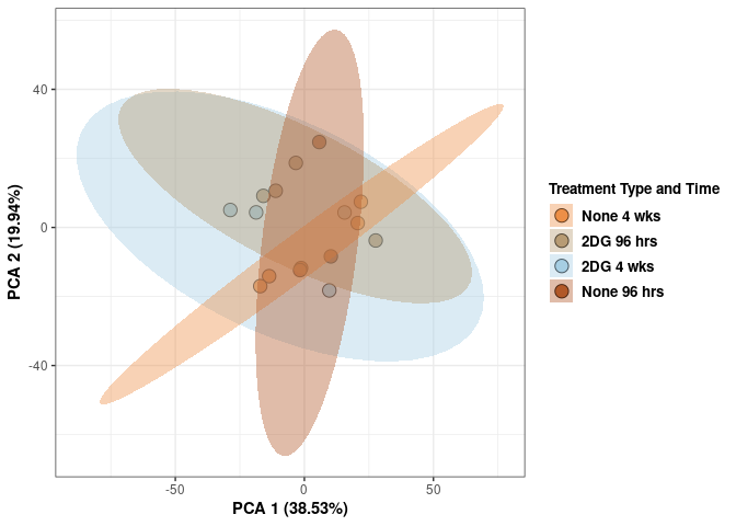
Treatment hypothalamus
Treatment_color <- as.factor(tdata.FPKM.sample.info.hypothalamus$Treatment)
Treatment_color <- as.data.frame(Treatment_color)
col_treatment <- colorRampPalette(brewer.pal(n = 12, name = "Paired"))(2)[Treatment_color$Treatment_color]
pca_treatment <- cbind(Treatment_color,pca$x[,1],pca$x[,2])
pca_treatment <- as.data.frame(pca_treatment)

p <- ggplot(pca_treatment,aes(pca$x[,1], pca$x[,2]))
p <- p + geom_point(aes(fill = as.factor(pca_treatment$Treatment_color)), shape=21, size=4) + theme_bw()
p <- p + theme(legend.title = element_text(size=10,face="bold")) +
  theme(legend.text = element_text(size=10, face="bold"))
p <- p + xlab("PCA 1 (38.53%)") + ylab("PCA 2 (19.94%)") + theme(axis.title = element_text(face="bold"))
p <- p + stat_ellipse(aes(pca$x[,1], pca$x[,2], group = Treatment_color, fill = as.factor(pca_treatment$Treatment_color)), geom="polygon",level=0.95,alpha=0.4) +
  scale_fill_manual(values=c("#A6CEE3", "#B15928"),name="Treatment Type",
                       breaks=c("2DG", "None"),
                       labels=c("2DG", "None")) +
  scale_linetype_manual(values=c(1,2))
print(p)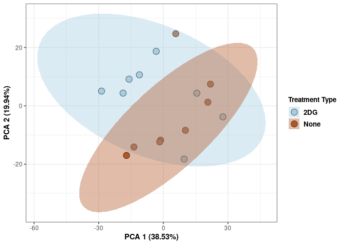
Time hypothalamus
Time_color <- as.factor(tdata.FPKM.sample.info.hypothalamus$Time)
Time_color <- as.data.frame(Time_color)
col_time <- colorRampPalette(brewer.pal(n = 12, name = "Paired"))(2)[Time_color$Time_color]
pca_time <- cbind(Time_color,pca$x[,1],pca$x[,2])
pca_time <- as.data.frame(pca_time)

p <- ggplot(pca_time,aes(pca$x[,1], pca$x[,2]))
p <- p + geom_point(aes(fill = as.factor(pca_time$Time_color)), shape=21, size=4) + theme_bw()
p <- p + theme(legend.title = element_text(size=10,face="bold")) +
  theme(legend.text = element_text(size=10, face="bold"))
p <- p + xlab("PCA 1 (38.53%)") + ylab("PCA 2 (19.94%)") + theme(axis.title = element_text(face="bold"))
p <- p + stat_ellipse(aes(pca$x[,1], pca$x[,2], group = Time_color, fill = as.factor(pca_time$Time_color)), geom="polygon",level=0.95,alpha=0.4) +
  scale_fill_manual(values=c("#A6CEE3", "#B15928"),name="Time",
                       breaks=c("4 wks", "96 hrs"),
                       labels=c("4 wks", "96 hrs")) +
  scale_linetype_manual(values=c(1,2))
print(p)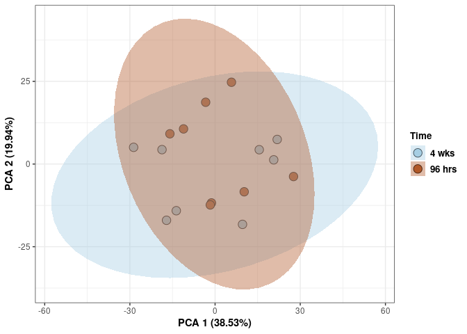
3D hypothalamus
This plot is color coded by time and treatment for hypothalamus, first collectively and then separately. To see each one click the names on the legend to make them disappear and click again to make them reappear.
Treatment_time_color <- as.factor(tdata.FPKM.sample.info.hypothalamus$treatment_time)
Treatment_time_color <- as.data.frame(Treatment_time_color)
col_treatment_time <- colorRampPalette(brewer.pal(n = 12, name = "Paired"))(4)[Treatment_time_color$Treatment_time_color]
pca_treatment_time <- cbind(Treatment_time_color,pca$x[,1],pca$x[,2],pca$x[,3])
pca_treatment_time <- as.data.frame(pca_treatment_time)
rownames(pca_treatment_time) <- rownames(tdata.FPKM.sample.info.hypothalamus)

p <- plot_ly(pca_treatment_time, x = pca_treatment_time$`pca$x[, 1]`, y = pca_treatment_time$`pca$x[, 2]`, z = pca_treatment_time$`pca$x[, 3]`, color = pca_treatment_time$Treatment_time_color, colors = c("#ED8F47", "#B89B74", "#A6CEE3", "#B15928"), text = rownames(pca_treatment_time)) %>%
  add_markers() %>%
  layout(scene = list(xaxis = list(title = "PC 1 27.09%"),
                     yaxis = list(title = "PC 2 16.01%"),
                     zaxis = list(title = "PC 3 6.69%")))

Treatment_color <- as.factor(tdata.FPKM.sample.info.hypothalamus$Treatment)
Treatment_color <- as.data.frame(Treatment_color)
col_treatment <- colorRampPalette(brewer.pal(n = 12, name = "Paired"))(2)[Treatment_color$Treatment_color]
pca_treatment <- cbind(Treatment_color,pca$x[,1],pca$x[,2],pca$x[,3])
pca_treatment <- as.data.frame(pca_treatment)
rownames(pca_treatment) <- rownames(tdata.FPKM.sample.info.hypothalamus)

p1 <- plot_ly(pca_treatment, x = pca_treatment$`pca$x[, 1]`, y = pca_treatment$`pca$x[, 2]`, z = pca_treatment$`pca$x[, 3]`, color = pca_treatment$Treatment_color, colors = c("#CC0000", "#330033"), text = rownames(pca_treatment)) %>%
  add_markers() %>%
  layout(scene = list(xaxis = list(title = "PC 1 27.09%"),
                     yaxis = list(title = "PC 2 16.01%"),
                     zaxis = list(title = "PC 3 6.69%")))

Time_color <- as.factor(tdata.FPKM.sample.info.hypothalamus$Time)
Time_color <- as.data.frame(Time_color)
col_time <- colorRampPalette(brewer.pal(n = 12, name = "Paired"))(2)[Time_color$Time_color]
pca_time <- cbind(Time_color,pca$x[,1],pca$x[,2],pca$x[,3])
pca_time <- as.data.frame(pca_time)
rownames(pca_time) <- rownames(tdata.FPKM.sample.info.hypothalamus)

p2 <- plot_ly(pca_time, x = pca_time$`pca$x[, 1]`, y = pca_time$`pca$x[, 2]`, z = pca_time$`pca$x[, 3]`, color = pca_time$Time_color, colors = c("#B8860B", "#00FA9A"), text = rownames(pca_time)) %>%
  add_markers() %>%
  layout(scene = list(xaxis = list(title = "PC 1 27.09%"),
                     yaxis = list(title = "PC 2 16.01%"),
                     zaxis = list(title = "PC 3 6.69%")))
p3 <- plotly::subplot(p,p1,p2)
p3
Scree plot and summary statistics hippocampus
tdata.FPKM.sample.info <- readRDS(here("Data","20190406_RNAseq_B6_4wk_2DG_counts_phenotypes.RData"))

tdata.FPKM.sample.info.hippocampus <- rownames_to_column(tdata.FPKM.sample.info) %>% filter(Tissue=="Hippocampus") %>% column_to_rownames('rowname')

tdata.FPKM <- readRDS(here("Data","20190406_RNAseq_B6_4wk_2DG_counts_numeric.RData"))

log.tdata.FPKM <- log(tdata.FPKM + 1)
log.tdata.FPKM <- as.data.frame(log.tdata.FPKM)

rows <- rownames(tdata.FPKM.sample.info.hippocampus)

log.tdata.FPKM.hippocampus <- rownames_to_column(log.tdata.FPKM)

log.tdata.FPKM.hippocampus <- log.tdata.FPKM.hippocampus %>% filter(rowname %in% rows) %>% column_to_rownames('rowname')

pca <- prcomp(log.tdata.FPKM.hippocampus, center = T)

screeplot(pca,type = "lines")
summary(pca)## Importance of components:
## PC1 PC2 PC3 PC4 PC5 PC6 PC7
## Standard deviation 20.1660 14.8302 12.9018 11.4249 10.78743 7.7869 6.78140
## Proportion of Variance 0.2938 0.1589 0.1202 0.0943 0.08407 0.0438 0.03322
## Cumulative Proportion 0.2938 0.4527 0.5729 0.6672 0.75129 0.7951 0.82831
## PC8 PC9 PC10 PC11 PC12 PC13 PC14
## Standard deviation 6.07067 5.79015 5.69394 5.66065 5.51625 5.08206 4.86288
## Proportion of Variance 0.02662 0.02422 0.02342 0.02315 0.02198 0.01866 0.01708
## Cumulative Proportion 0.85494 0.87916 0.90258 0.92573 0.94771 0.96637 0.98345
## PC15 PC16
## Standard deviation 4.78623 1.639e-14
## Proportion of Variance 0.01655 0.000e+00
## Cumulative Proportion 1.00000 1.000e+00Treatment and time hippocampus
tdata.FPKM.sample.info <- readRDS(here("Data","20190406_RNAseq_B6_4wk_2DG_counts_phenotypes.RData"))

treatment_time <-paste(tdata.FPKM.sample.info$Treatment, tdata.FPKM.sample.info$Time)

tdata.FPKM.sample.info <-cbind(tdata.FPKM.sample.info,treatment_time)

tdata.FPKM.sample.info.hippocampus <- rownames_to_column(tdata.FPKM.sample.info) %>% filter(Tissue=="Hippocampus") %>% column_to_rownames('rowname')

tdata.FPKM <- readRDS(here("Data","20190406_RNAseq_B6_4wk_2DG_counts_numeric.RData"))

log.tdata.FPKM <- log(tdata.FPKM + 1)
log.tdata.FPKM <- as.data.frame(log.tdata.FPKM)

rows <- rownames(tdata.FPKM.sample.info.hippocampus)

log.tdata.FPKM.hippocampus <- rownames_to_column(log.tdata.FPKM)

log.tdata.FPKM.hippocampus <- log.tdata.FPKM.hippocampus %>% filter(rowname %in% rows) %>% column_to_rownames('rowname')

pca <- prcomp(log.tdata.FPKM.hippocampus, center = T)

screeplot(pca,type = "lines")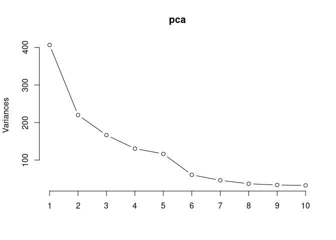
summary(pca)## Importance of components:
## PC1 PC2 PC3 PC4 PC5 PC6 PC7
## Standard deviation 20.1660 14.8302 12.9018 11.4249 10.78743 7.7869 6.78140
## Proportion of Variance 0.2938 0.1589 0.1202 0.0943 0.08407 0.0438 0.03322
## Cumulative Proportion 0.2938 0.4527 0.5729 0.6672 0.75129 0.7951 0.82831
## PC8 PC9 PC10 PC11 PC12 PC13 PC14
## Standard deviation 6.07067 5.79015 5.69394 5.66065 5.51625 5.08206 4.86288
## Proportion of Variance 0.02662 0.02422 0.02342 0.02315 0.02198 0.01866 0.01708
## Cumulative Proportion 0.85494 0.87916 0.90258 0.92573 0.94771 0.96637 0.98345
## PC15 PC16
## Standard deviation 4.78623 1.639e-14
## Proportion of Variance 0.01655 0.000e+00
## Cumulative Proportion 1.00000 1.000e+00Treatment_time_color <- as.factor(tdata.FPKM.sample.info.hippocampus$treatment_time)
Treatment_time_color <- as.data.frame(Treatment_time_color)
col_treatment_time <- colorRampPalette(brewer.pal(n = 12, name = "Paired"))(4)[Treatment_time_color$Treatment_time_color]
pca_treatment_time <- cbind(Treatment_time_color,pca$x[,1],pca$x[,2])
pca_treatment_time <- as.data.frame(pca_treatment_time)
p <- ggplot(pca_treatment_time,aes(pca$x[,1], pca$x[,2]))
p <- p + geom_point(aes(fill = as.factor(pca_treatment_time$Treatment_time_color)), shape=21, size=4) + theme_bw()
p <- p + theme(legend.title = element_text(size=10,face="bold")) +
theme(legend.text = element_text(size=10, face="bold"))
p <- p + xlab("PCA 1 (29.38%)") + ylab("PCA 2 (15.89%)") + theme(axis.title = element_text(face="bold"))
p <- p + stat_ellipse(aes(pca$x[,1], pca$x[,2], group = Treatment_time_color, fill = as.factor(pca_treatment_time$Treatment_time_color)), geom="polygon",level=0.95,alpha=0.4) +
scale_fill_manual(values=c("#ED8F47", "#B89B74", "#A6CEE3", "#B15928"),name="Treatment Type and Time",
breaks=c("None 4 wks", "2DG 96 hrs", "2DG 4 wks", "None 96 hrs"),
labels=c("None 4 wks", "2DG 96 hrs", "2DG 4 wks", "None 96 hrs")) +
scale_linetype_manual(values=c(1,2))
print(p)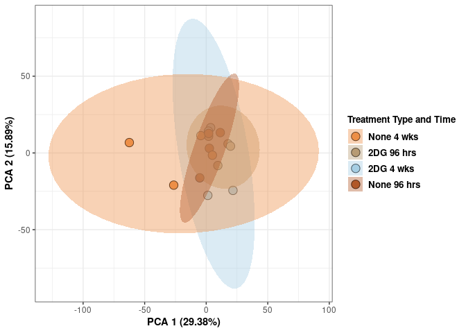
Treatment hippocampus
Treatment_color <- as.factor(tdata.FPKM.sample.info.hippocampus$Treatment)
Treatment_color <- as.data.frame(Treatment_color)
col_treatment <- colorRampPalette(brewer.pal(n = 12, name = "Paired"))(2)[Treatment_color$Treatment_color]
pca_treatment <- cbind(Treatment_color,pca$x[,1],pca$x[,2])
pca_treatment <- as.data.frame(pca_treatment)

p <- ggplot(pca_treatment,aes(pca$x[,1], pca$x[,2]))
p <- p + geom_point(aes(fill = as.factor(pca_treatment$Treatment_color)), shape=21, size=4) + theme_bw()
p <- p + theme(legend.title = element_text(size=10,face="bold")) +
  theme(legend.text = element_text(size=10, face="bold"))
p <- p + xlab("PCA 1 (29.38%)") + ylab("PCA 2 (15.89%)") + theme(axis.title = element_text(face="bold"))
p <- p + stat_ellipse(aes(pca$x[,1], pca$x[,2], group = Treatment_color, fill = as.factor(pca_treatment$Treatment_color)), geom="polygon",level=0.95,alpha=0.4) +
  scale_fill_manual(values=c("#A6CEE3", "#B15928"),name="Treatment Type",
                       breaks=c("2DG", "None"),
                       labels=c("2DG", "None")) +
  scale_linetype_manual(values=c(1,2))
print(p)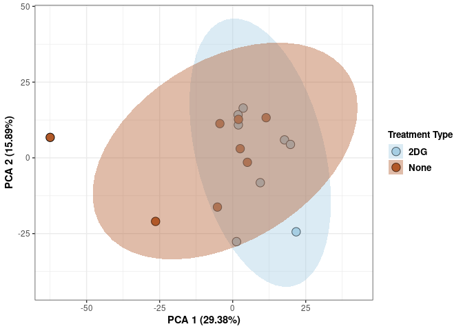
Time hippocampus
Time_color <- as.factor(tdata.FPKM.sample.info.hippocampus$Time)
Time_color <- as.data.frame(Time_color)
col_time <- colorRampPalette(brewer.pal(n = 12, name = "Paired"))(2)[Time_color$Time_color]
pca_time <- cbind(Time_color,pca$x[,1],pca$x[,2])
pca_time <- as.data.frame(pca_time)

p <- ggplot(pca_time,aes(pca$x[,1], pca$x[,2]))
p <- p + geom_point(aes(fill = as.factor(pca_time$Time_color)), shape=21, size=4) + theme_bw()
p <- p + theme(legend.title = element_text(size=10,face="bold")) +
  theme(legend.text = element_text(size=10, face="bold"))
p <- p + xlab("PCA 1 (38.53%)") + ylab("PCA 2 (19.94%)") + theme(axis.title = element_text(face="bold"))
p <- p + stat_ellipse(aes(pca$x[,1], pca$x[,2], group = Time_color, fill = as.factor(pca_time$Time_color)), geom="polygon",level=0.95,alpha=0.4) +
  scale_fill_manual(values=c("#A6CEE3", "#B15928"),name="Time",
                       breaks=c("4 wks", "96 hrs"),
                       labels=c("4 wks", "96 hrs")) +
  scale_linetype_manual(values=c(1,2))
print(p)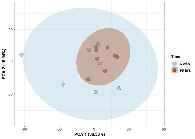
3D hippocampus
This plot is color coded by time and treatment for hippocampus, first collectively and then separately. To see each one click the names on the legend to make them disappear and click again to make them reappear.
Treatment_time_color <- as.factor(tdata.FPKM.sample.info.hippocampus$treatment_time)
Treatment_time_color <- as.data.frame(Treatment_time_color)
col_treatment_time <- colorRampPalette(brewer.pal(n = 12, name = "Paired"))(4)[Treatment_time_color$Treatment_time_color]
pca_treatment_time <- cbind(Treatment_time_color,pca$x[,1],pca$x[,2], pca$x[,3])
pca_treatment_time <- as.data.frame(pca_treatment_time)
rownames(pca_treatment_time) <- rownames(tdata.FPKM.sample.info.hippocampus)

p <- plot_ly(pca_treatment_time, x = pca_treatment_time$`pca$x[, 1]`, y = pca_treatment_time$`pca$x[, 2]`, z = pca_treatment_time$`pca$x[, 3]`, color = pca_treatment_time$Treatment_time_color, colors = c("#ED8F47", "#B89B74", "#A6CEE3", "#B15928"), text = rownames(pca_treatment_time)) %>%
  add_markers() %>%
  layout(scene = list(xaxis = list(title = "PC 1 29.38%"),
                     yaxis = list(title = "PC 2 15.89%"),
                     zaxis = list(title = "PC 3 12.02%")))

Treatment_color <- as.factor(tdata.FPKM.sample.info.hippocampus$Treatment)
Treatment_color <- as.data.frame(Treatment_color)
col_treatment <- colorRampPalette(brewer.pal(n = 12, name = "Paired"))(2)[Treatment_color$Treatment_color]
pca_treatment <- cbind(Treatment_color,pca$x[,1],pca$x[,2],pca$x[,3])
pca_treatment <- as.data.frame(pca_treatment)
rownames(pca_treatment) <- rownames(tdata.FPKM.sample.info.hippocampus)

p1 <- plot_ly(pca_treatment, x = pca_treatment$`pca$x[, 1]`, y = pca_treatment$`pca$x[, 2]`, z = pca_treatment$`pca$x[, 3]`, color = pca_treatment$Treatment_color, colors = c("#CC0000", "#330033"), text = rownames(pca_treatment)) %>%
  add_markers() %>%
  layout(scene = list(xaxis = list(title = "PC 1 29.38%"),
                     yaxis = list(title = "PC 2 15.89%"),
                     zaxis = list(title = "PC 3 12.02%")))

Time_color <- as.factor(tdata.FPKM.sample.info.hippocampus$Time)
Time_color <- as.data.frame(Time_color)
col_time <- colorRampPalette(brewer.pal(n = 12, name = "Paired"))(2)[Time_color$Time_color]
pca_time <- cbind(Time_color,pca$x[,1],pca$x[,2],pca$x[,3])
pca_time <- as.data.frame(pca_time)
rownames(pca_time) <- rownames(tdata.FPKM.sample.info.hippocampus)

p2 <- plot_ly(pca_time, x = pca_time$`pca$x[, 1]`, y = pca_time$`pca$x[, 2]`, z = pca_time$`pca$x[, 3]`, color = pca_time$Time_color, colors = c("#B8860B", "#00FA9A"), text = rownames(pca_time)) %>%
  add_markers() %>%
  layout(scene = list(xaxis = list(title = "PC 1 29.38%"),
                     yaxis = list(title = "PC 2 15.89%"),
                     zaxis = list(title = "PC 3 12.02%")))
p3 <- plotly::subplot(p,p1,p2)
p3
Scree plot and summary statistics liver
tdata.FPKM.sample.info <- readRDS(here("Data","20190406_RNAseq_B6_4wk_2DG_counts_phenotypes.RData"))

tdata.FPKM.sample.info.liver <- rownames_to_column(tdata.FPKM.sample.info) %>% filter(Tissue=="Liver") %>% column_to_rownames('rowname')

tdata.FPKM <- readRDS(here("Data","20190406_RNAseq_B6_4wk_2DG_counts_numeric.RData"))

log.tdata.FPKM <- log(tdata.FPKM + 1)
log.tdata.FPKM <- as.data.frame(log.tdata.FPKM)

rows <- rownames(tdata.FPKM.sample.info.liver)

log.tdata.FPKM.liver <- rownames_to_column(log.tdata.FPKM)

log.tdata.FPKM.liver <- log.tdata.FPKM.liver %>% filter(rowname %in% rows) %>% column_to_rownames('rowname')

pca <- prcomp(log.tdata.FPKM.liver, center = T)

screeplot(pca,type = "lines")
summary(pca)## Importance of components:
## PC1 PC2 PC3 PC4 PC5 PC6 PC7
## Standard deviation 15.9033 9.9879 8.2469 7.62761 7.05632 6.87169 6.55218
## Proportion of Variance 0.2979 0.1175 0.0801 0.06852 0.05864 0.05561 0.05056
## Cumulative Proportion 0.2979 0.4153 0.4955 0.56397 0.62261 0.67822 0.72879
## PC8 PC9 PC10 PC11 PC12 PC13 PC14
## Standard deviation 6.04350 5.74564 5.61541 5.43365 5.25537 5.01913 4.96453
## Proportion of Variance 0.04302 0.03888 0.03714 0.03477 0.03253 0.02967 0.02903
## Cumulative Proportion 0.77180 0.81068 0.84782 0.88259 0.91512 0.94478 0.97381
## PC15 PC16
## Standard deviation 4.71554 1.361e-14
## Proportion of Variance 0.02619 0.000e+00
## Cumulative Proportion 1.00000 1.000e+00Treatment and time liver
tdata.FPKM.sample.info <- readRDS(here("Data","20190406_RNAseq_B6_4wk_2DG_counts_phenotypes.RData"))

treatment_time <-paste(tdata.FPKM.sample.info$Treatment, tdata.FPKM.sample.info$Time)

tdata.FPKM.sample.info <-cbind(tdata.FPKM.sample.info,treatment_time)

tdata.FPKM.sample.info.liver <- rownames_to_column(tdata.FPKM.sample.info) %>% filter(Tissue=="Liver") %>% column_to_rownames('rowname')

tdata.FPKM <- readRDS(here("Data","20190406_RNAseq_B6_4wk_2DG_counts_numeric.RData"))

log.tdata.FPKM <- log(tdata.FPKM + 1)
log.tdata.FPKM <- as.data.frame(log.tdata.FPKM)

rows <- rownames(tdata.FPKM.sample.info.liver)

log.tdata.FPKM.liver <- rownames_to_column(log.tdata.FPKM)

log.tdata.FPKM.liver <- log.tdata.FPKM.liver %>% filter(rowname %in% rows) %>% column_to_rownames('rowname')

pca <- prcomp(log.tdata.FPKM.liver, center = T)

screeplot(pca,type = "lines")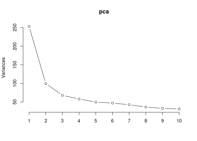
summary(pca)## Importance of components:
## PC1 PC2 PC3 PC4 PC5 PC6 PC7
## Standard deviation 15.9033 9.9879 8.2469 7.62761 7.05632 6.87169 6.55218
## Proportion of Variance 0.2979 0.1175 0.0801 0.06852 0.05864 0.05561 0.05056
## Cumulative Proportion 0.2979 0.4153 0.4955 0.56397 0.62261 0.67822 0.72879
## PC8 PC9 PC10 PC11 PC12 PC13 PC14
## Standard deviation 6.04350 5.74564 5.61541 5.43365 5.25537 5.01913 4.96453
## Proportion of Variance 0.04302 0.03888 0.03714 0.03477 0.03253 0.02967 0.02903
## Cumulative Proportion 0.77180 0.81068 0.84782 0.88259 0.91512 0.94478 0.97381
## PC15 PC16
## Standard deviation 4.71554 1.361e-14
## Proportion of Variance 0.02619 0.000e+00
## Cumulative Proportion 1.00000 1.000e+00Treatment_time_color <- as.factor(tdata.FPKM.sample.info.liver$treatment_time)
Treatment_time_color <- as.data.frame(Treatment_time_color)
col_treatment_time <- colorRampPalette(brewer.pal(n = 12, name = "Paired"))(4)[Treatment_time_color$Treatment_time_color]
pca_treatment_time <- cbind(Treatment_time_color,pca$x[,1],pca$x[,2])
pca_treatment_time <- as.data.frame(pca_treatment_time)
p <- ggplot(pca_treatment_time,aes(pca$x[,1], pca$x[,2]))
p <- p + geom_point(aes(fill = as.factor(pca_treatment_time$Treatment_time_color)), shape=21, size=4) + theme_bw()
p <- p + theme(legend.title = element_text(size=10,face="bold")) +
theme(legend.text = element_text(size=10, face="bold"))
p <- p + xlab("PCA 1 (29.79%)") + ylab("PCA 2 (11.75%)") + theme(axis.title = element_text(face="bold"))
p <- p + stat_ellipse(aes(pca$x[,1], pca$x[,2], group = Treatment_time_color, fill = as.factor(pca_treatment_time$Treatment_time_color)), geom="polygon",level=0.95,alpha=0.4) +
scale_fill_manual(values=c("#ED8F47", "#B89B74", "#A6CEE3", "#B15928"),name="Treatment Type and Time",
breaks=c("None 4 wks", "2DG 96 hrs", "2DG 4 wks", "None 96 hrs"),
labels=c("None 4 wks", "2DG 96 hrs", "2DG 4 wks", "None 96 hrs")) +
scale_linetype_manual(values=c(1,2))
print(p)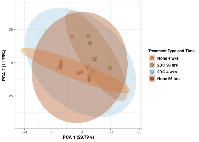
Treatment liver
Treatment_color <- as.factor(tdata.FPKM.sample.info.liver$Treatment)
Treatment_color <- as.data.frame(Treatment_color)
col_treatment <- colorRampPalette(brewer.pal(n = 12, name = "Paired"))(2)[Treatment_color$Treatment_color]
pca_treatment <- cbind(Treatment_color,pca$x[,1],pca$x[,2])
pca_treatment <- as.data.frame(pca_treatment)

p <- ggplot(pca_treatment,aes(pca$x[,1], pca$x[,2]))
p <- p + geom_point(aes(fill = as.factor(pca_treatment$Treatment_color)), shape=21, size=4) + theme_bw()
p <- p + theme(legend.title = element_text(size=10,face="bold")) +
  theme(legend.text = element_text(size=10, face="bold"))
p <- p + xlab("PCA 1 (38.53%)") + ylab("PCA 2 (19.94%)") + theme(axis.title = element_text(face="bold"))
p <- p + stat_ellipse(aes(pca$x[,1], pca$x[,2], group = Treatment_color, fill = as.factor(pca_treatment$Treatment_color)), geom="polygon",level=0.95,alpha=0.4) +
  scale_fill_manual(values=c("#A6CEE3", "#B15928"),name="Treatment Type",
                       breaks=c("2DG", "None"),
                       labels=c("2DG", "None")) +
  scale_linetype_manual(values=c(1,2))
print(p)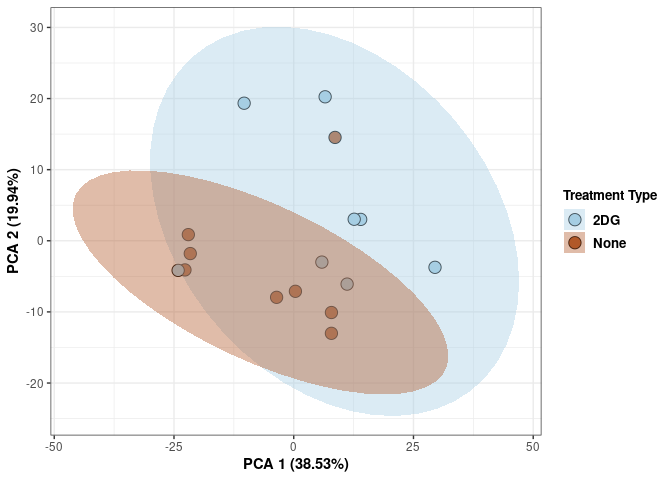
Time liver
Time_color <- as.factor(tdata.FPKM.sample.info.liver$Time)
Time_color <- as.data.frame(Time_color)
col_time <- colorRampPalette(brewer.pal(n = 12, name = "Paired"))(2)[Time_color$Time_color]
pca_time <- cbind(Time_color,pca$x[,1],pca$x[,2])
pca_time <- as.data.frame(pca_time)

p <- ggplot(pca_time,aes(pca$x[,1], pca$x[,2]))
p <- p + geom_point(aes(fill = as.factor(pca_time$Time_color)), shape=21, size=4) + theme_bw()
p <- p + theme(legend.title = element_text(size=10,face="bold")) +
  theme(legend.text = element_text(size=10, face="bold"))
p <- p + xlab("PCA 1 (38.53%)") + ylab("PCA 2 (19.94%)") + theme(axis.title = element_text(face="bold"))
p <- p + stat_ellipse(aes(pca$x[,1], pca$x[,2], group = Time_color, fill = as.factor(pca_time$Time_color)), geom="polygon",level=0.95,alpha=0.4) +
  scale_fill_manual(values=c("#A6CEE3", "#B15928"),name="Time",
                       breaks=c("4 wks", "96 hrs"),
                       labels=c("4 wks", "96 hrs")) +
  scale_linetype_manual(values=c(1,2))
print(p)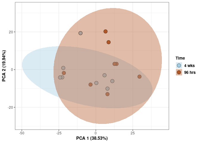
3D liver
This plot is color coded by time and treatment for liver, first collectively and then separately. To see each one click the names on the legend to make them disappear and click again to make them reappear.
Treatment_time_color <- as.factor(tdata.FPKM.sample.info.liver$treatment_time)
Treatment_time_color <- as.data.frame(Treatment_time_color)
col_treatment_time <- colorRampPalette(brewer.pal(n = 12, name = "Paired"))(4)[Treatment_time_color$Treatment_time_color]
pca_treatment_time <- cbind(Treatment_time_color,pca$x[,1],pca$x[,2],pca$x[,3])
pca_treatment_time <- as.data.frame(pca_treatment_time)
rownames(pca_treatment_time) <- rownames(tdata.FPKM.sample.info.liver)

p <- plot_ly(pca_treatment_time, x = pca_treatment_time$`pca$x[, 1]`, y = pca_treatment_time$`pca$x[, 2]`, z = pca_treatment_time$`pca$x[, 3]`, color = pca_treatment_time$Treatment_time_color, colors = c("#ED8F47", "#B89B74", "#A6CEE3", "#B15928"), text = rownames(pca_treatment_time)) %>%
  add_markers() %>%
  layout(scene = list(xaxis = list(title = "PC 1 29.79%"),
                     yaxis = list(title = "PC 2 11.75%"),
                     zaxis = list(title = "PC 3 8.01%")))

Treatment_color <- as.factor(tdata.FPKM.sample.info.liver$Treatment)
Treatment_color <- as.data.frame(Treatment_color)
col_treatment <- colorRampPalette(brewer.pal(n = 12, name = "Paired"))(2)[Treatment_color$Treatment_color]
pca_treatment <- cbind(Treatment_color,pca$x[,1],pca$x[,2],pca$x[,3])
pca_treatment <- as.data.frame(pca_treatment)
rownames(pca_treatment) <- rownames(tdata.FPKM.sample.info.liver)

p1 <- plot_ly(pca_treatment, x = pca_treatment$`pca$x[, 1]`, y = pca_treatment$`pca$x[, 2]`, z = pca_treatment$`pca$x[, 3]`, color = pca_treatment$Treatment_color, colors = c("#CC0000", "#330033"), text = rownames(pca_treatment)) %>%
  add_markers() %>%
  layout(scene = list(xaxis = list(title = "PC 1 29.79%"),
                     yaxis = list(title = "PC 2 11.75%"),
                     zaxis = list(title = "PC 3 8.01%")))

Time_color <- as.factor(tdata.FPKM.sample.info.liver$Time)
Time_color <- as.data.frame(Time_color)
col_time <- colorRampPalette(brewer.pal(n = 12, name = "Paired"))(2)[Time_color$Time_color]
pca_time <- cbind(Time_color,pca$x[,1],pca$x[,2],pca$x[,3])
pca_time <- as.data.frame(pca_time)
rownames(pca_time) <- rownames(tdata.FPKM.sample.info.liver)

p2 <- plot_ly(pca_time, x = pca_time$`pca$x[, 1]`, y = pca_time$`pca$x[, 2]`, z = pca_time$`pca$x[, 3]`, color = pca_time$Time_color, colors = c("#B8860B", "#00FA9A"), text = rownames(pca_time)) %>%
  add_markers() %>%
  layout(scene = list(xaxis = list(title = "PC 1 29.79%"),
                     yaxis = list(title = "PC 2 11.75%"),
                     zaxis = list(title = "PC 3 8.01%")))
p3 <- plotly::subplot(p,p1,p2)
p3
Scree plot and summary statistics heart
tdata.FPKM.sample.info <- readRDS(here("Data","20190406_RNAseq_B6_4wk_2DG_counts_phenotypes.RData"))

tdata.FPKM.sample.info.heart <- rownames_to_column(tdata.FPKM.sample.info) %>% filter(Tissue=="Heart") %>% column_to_rownames('rowname')

tdata.FPKM <- readRDS(here("Data","20190406_RNAseq_B6_4wk_2DG_counts_numeric.RData"))

log.tdata.FPKM <- log(tdata.FPKM + 1)
log.tdata.FPKM <- as.data.frame(log.tdata.FPKM)

rows <- rownames(tdata.FPKM.sample.info.heart)

log.tdata.FPKM.heart <- rownames_to_column(log.tdata.FPKM)

log.tdata.FPKM.heart <- log.tdata.FPKM.heart %>% filter(rowname %in% rows) %>% column_to_rownames('rowname')

pca <- prcomp(log.tdata.FPKM.heart, center = T)

screeplot(pca,type = "lines")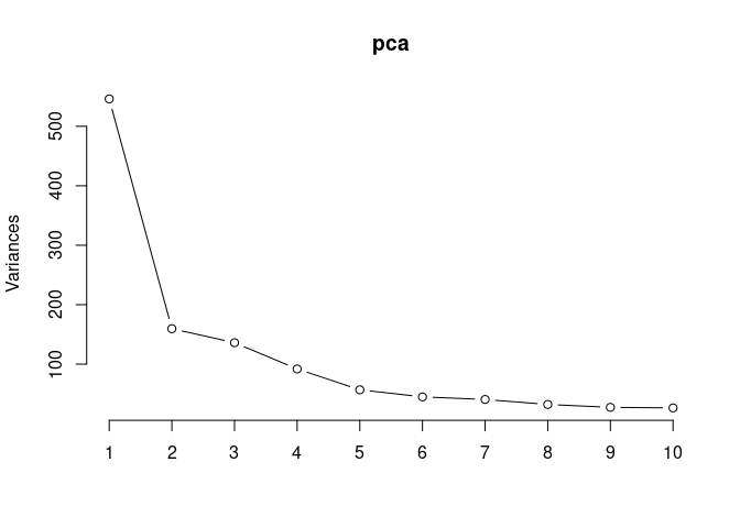
summary(pca)## Importance of components:
## PC1 PC2 PC3 PC4 PC5 PC6 PC7
## Standard deviation 23.368 12.6331 11.6620 9.58496 7.53532 6.70152 6.36958
## Proportion of Variance 0.429 0.1254 0.1069 0.07218 0.04461 0.03528 0.03187
## Cumulative Proportion 0.429 0.5544 0.6612 0.73340 0.77801 0.81329 0.84516
## PC8 PC9 PC10 PC11 PC12 PC13 PC14
## Standard deviation 5.67280 5.22830 5.13213 5.07854 4.94706 4.6924 4.47873
## Proportion of Variance 0.02528 0.02148 0.02069 0.02026 0.01923 0.0173 0.01576
## Cumulative Proportion 0.87045 0.89192 0.91261 0.93287 0.95210 0.9694 0.98516
## PC15 PC16
## Standard deviation 4.34635 1.289e-14
## Proportion of Variance 0.01484 0.000e+00
## Cumulative Proportion 1.00000 1.000e+00Treatment and time heart
tdata.FPKM.sample.info <- readRDS(here("Data","20190406_RNAseq_B6_4wk_2DG_counts_phenotypes.RData"))

treatment_time <-paste(tdata.FPKM.sample.info$Treatment, tdata.FPKM.sample.info$Time)

tdata.FPKM.sample.info <-cbind(tdata.FPKM.sample.info,treatment_time)

tdata.FPKM.sample.info.heart <- rownames_to_column(tdata.FPKM.sample.info) %>% filter(Tissue=="Heart") %>% column_to_rownames('rowname')

tdata.FPKM <- readRDS(here("Data","20190406_RNAseq_B6_4wk_2DG_counts_numeric.RData"))

log.tdata.FPKM <- log(tdata.FPKM + 1)
log.tdata.FPKM <- as.data.frame(log.tdata.FPKM)

rows <- rownames(tdata.FPKM.sample.info.heart)

log.tdata.FPKM.heart <- rownames_to_column(log.tdata.FPKM)

log.tdata.FPKM.heart <- log.tdata.FPKM.heart %>% filter(rowname %in% rows) %>% column_to_rownames('rowname')

pca <- prcomp(log.tdata.FPKM.heart, center = T)

screeplot(pca,type = "lines")
summary(pca)## Importance of components:
## PC1 PC2 PC3 PC4 PC5 PC6 PC7
## Standard deviation 23.368 12.6331 11.6620 9.58496 7.53532 6.70152 6.36958
## Proportion of Variance 0.429 0.1254 0.1069 0.07218 0.04461 0.03528 0.03187
## Cumulative Proportion 0.429 0.5544 0.6612 0.73340 0.77801 0.81329 0.84516
## PC8 PC9 PC10 PC11 PC12 PC13 PC14
## Standard deviation 5.67280 5.22830 5.13213 5.07854 4.94706 4.6924 4.47873
## Proportion of Variance 0.02528 0.02148 0.02069 0.02026 0.01923 0.0173 0.01576
## Cumulative Proportion 0.87045 0.89192 0.91261 0.93287 0.95210 0.9694 0.98516
## PC15 PC16
## Standard deviation 4.34635 1.289e-14
## Proportion of Variance 0.01484 0.000e+00
## Cumulative Proportion 1.00000 1.000e+00Treatment_time_color <- as.factor(tdata.FPKM.sample.info.heart$treatment_time)
Treatment_time_color <- as.data.frame(Treatment_time_color)
col_treatment_time <- colorRampPalette(brewer.pal(n = 12, name = "Paired"))(4)[Treatment_time_color$Treatment_time_color]
pca_treatment_time <- cbind(Treatment_time_color,pca$x[,1],pca$x[,2])
pca_treatment_time <- as.data.frame(pca_treatment_time)
p <- ggplot(pca_treatment_time,aes(pca$x[,1], pca$x[,2]))
p <- p + geom_point(aes(fill = as.factor(pca_treatment_time$Treatment_time_color)), shape=21, size=4) + theme_bw()
p <- p + theme(legend.title = element_text(size=10,face="bold")) +
theme(legend.text = element_text(size=10, face="bold"))
p <- p + xlab("PCA 1 (42.9%)") + ylab("PCA 2 (12.54%)") + theme(axis.title = element_text(face="bold"))
p <- p + stat_ellipse(aes(pca$x[,1], pca$x[,2], group = Treatment_time_color, fill = as.factor(pca_treatment_time$Treatment_time_color)), geom="polygon",level=0.95,alpha=0.4) +
scale_fill_manual(values=c("#ED8F47", "#B89B74", "#A6CEE3", "#B15928"),name="Treatment Type and Time",
breaks=c("None 4 wks", "2DG 96 hrs", "2DG 4 wks", "None 96 hrs"),
labels=c("None 4 wks", "2DG 96 hrs", "2DG 4 wks", "None 96 hrs")) +
scale_linetype_manual(values=c(1,2))
print(p)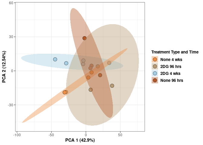
Treatment heart
Treatment_color <- as.factor(tdata.FPKM.sample.info.heart$Treatment)
Treatment_color <- as.data.frame(Treatment_color)
col_treatment <- colorRampPalette(brewer.pal(n = 12, name = "Paired"))(2)[Treatment_color$Treatment_color]
pca_treatment <- cbind(Treatment_color,pca$x[,1],pca$x[,2])
pca_treatment <- as.data.frame(pca_treatment)

p <- ggplot(pca_treatment,aes(pca$x[,1], pca$x[,2]))
p <- p + geom_point(aes(fill = as.factor(pca_treatment$Treatment_color)), shape=21, size=4) + theme_bw()
p <- p + theme(legend.title = element_text(size=10,face="bold")) +
  theme(legend.text = element_text(size=10, face="bold"))
p <- p + xlab("PCA 1 (42.9%)") + ylab("PCA 2 (12.54%)") + theme(axis.title = element_text(face="bold"))
p <- p + stat_ellipse(aes(pca$x[,1], pca$x[,2], group = Treatment_color, fill = as.factor(pca_treatment$Treatment_color)), geom="polygon",level=0.95,alpha=0.4) +
  scale_fill_manual(values=c("#A6CEE3", "#B15928"),name="Treatment Type",
                       breaks=c("2DG", "None"),
                       labels=c("2DG", "heart")) +
  scale_linetype_manual(values=c(1,2))
print(p)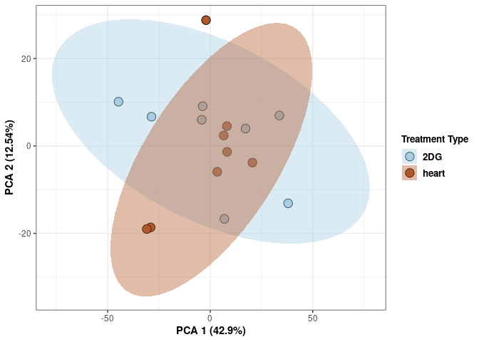
Time heart
Time_color <- as.factor(tdata.FPKM.sample.info.heart$Time)
Time_color <- as.data.frame(Time_color)
col_time <- colorRampPalette(brewer.pal(n = 12, name = "Paired"))(2)[Time_color$Time_color]
pca_time <- cbind(Time_color,pca$x[,1],pca$x[,2])
pca_time <- as.data.frame(pca_time)

p <- ggplot(pca_time,aes(pca$x[,1], pca$x[,2]))
p <- p + geom_point(aes(fill = as.factor(pca_time$Time_color)), shape=21, size=4) + theme_bw()
p <- p + theme(legend.title = element_text(size=10,face="bold")) +
  theme(legend.text = element_text(size=10, face="bold"))
p <- p + xlab("PCA 1 (42.9%)") + ylab("PCA 2 (12.54%)") + theme(axis.title = element_text(face="bold"))
p <- p + stat_ellipse(aes(pca$x[,1], pca$x[,2], group = Time_color, fill = as.factor(pca_time$Time_color)), geom="polygon",level=0.95,alpha=0.4) +
  scale_fill_manual(values=c("#A6CEE3", "#B15928"),name="Time",
                       breaks=c("4 wks", "96 hrs"),
                       labels=c("4 wks", "96 hrs")) +
  scale_linetype_manual(values=c(1,2))
print(p)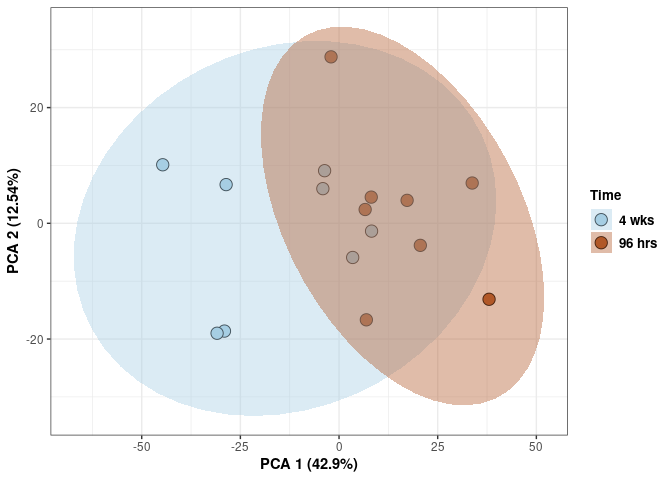
3D heart
This plot is color coded by time and treatment for heart, first collectively and then separately. To see each one click the names on the legend to make them disappear and click again to make them reappear.
Treatment_time_color <- as.factor(tdata.FPKM.sample.info.heart$treatment_time)
Treatment_time_color <- as.data.frame(Treatment_time_color)
col_treatment_time <- colorRampPalette(brewer.pal(n = 12, name = "Paired"))(4)[Treatment_time_color$Treatment_time_color]
pca_treatment_time <- cbind(Treatment_time_color,pca$x[,1],pca$x[,2],pca$x[,3])
pca_treatment_time <- as.data.frame(pca_treatment_time)
rownames(pca_treatment_time) <- rownames(tdata.FPKM.sample.info.heart)

p <- plot_ly(pca_treatment_time, x = pca_treatment_time$`pca$x[, 1]`, y = pca_treatment_time$`pca$x[, 2]`, z = pca_treatment_time$`pca$x[, 3]`, color = pca_treatment_time$Treatment_time_color, colors = c("#ED8F47", "#B89B74", "#A6CEE3", "#B15928"), text = rownames(pca_treatment_time)) %>%
  add_markers() %>%
  layout(scene = list(xaxis = list(title = "PC 1 42.9%"),
                     yaxis = list(title = "PC 2 12.54%"),
                     zaxis = list(title = "PC 3 10.69%")))

Treatment_color <- as.factor(tdata.FPKM.sample.info.heart$Treatment)
Treatment_color <- as.data.frame(Treatment_color)
col_treatment <- colorRampPalette(brewer.pal(n = 12, name = "Paired"))(2)[Treatment_color$Treatment_color]
pca_treatment <- cbind(Treatment_color,pca$x[,1],pca$x[,2],pca$x[,3])
rownames(pca_treatment) <- rownames(tdata.FPKM.sample.info.heart)

p1 <- plot_ly(pca_treatment, x = pca_treatment$`pca$x[, 1]`, y = pca_treatment$`pca$x[, 2]`, z = pca_treatment$`pca$x[, 3]`, color = pca_treatment$Treatment_color, colors = c("#CC0000", "#330033"), text = rownames(pca_treatment)) %>%
  add_markers() %>%
  layout(scene = list(xaxis = list(title = "PC 1 42.9%"),
                     yaxis = list(title = "PC 2 12.54%"),
                     zaxis = list(title = "PC 3 10.69%")))

Time_color <- as.factor(tdata.FPKM.sample.info.heart$Time)
Time_color <- as.data.frame(Time_color)
col_time <- colorRampPalette(brewer.pal(n = 12, name = "Paired"))(2)[Time_color$Time_color]
pca_time <- cbind(Time_color,pca$x[,1],pca$x[,2],pca$x[,3])
rownames(pca_time) <- rownames(tdata.FPKM.sample.info.heart)

p2 <- plot_ly(pca_time, x = pca_time$`pca$x[, 1]`, y = pca_time$`pca$x[, 2]`, z = pca_time$`pca$x[, 3]`, color = pca_time$Time_color, colors = c("#B8860B", "#00FA9A"), text = rownames(pca_time)) %>%
  add_markers() %>%
  layout(scene = list(xaxis = list(title = "PC 1 42.9%"),
                     yaxis = list(title = "PC 2 12.54%"),
                     zaxis = list(title = "PC 3 10.69%")))
p3 <- plotly::subplot(p,p1,p2)
p3
Scree plot and summary statistics small intestine
tdata.FPKM.sample.info <- readRDS(here("Data","20190406_RNAseq_B6_4wk_2DG_counts_phenotypes.RData"))

tdata.FPKM.sample.info.small.intestine <- rownames_to_column(tdata.FPKM.sample.info) %>% filter(Tissue=="Small Intestine") %>% column_to_rownames('rowname')

tdata.FPKM <- readRDS(here("Data","20190406_RNAseq_B6_4wk_2DG_counts_numeric.RData"))

log.tdata.FPKM <- log(tdata.FPKM + 1)
log.tdata.FPKM <- as.data.frame(log.tdata.FPKM)

rows <- rownames(tdata.FPKM.sample.info.small.intestine)

log.tdata.FPKM.small.intestine <- rownames_to_column(log.tdata.FPKM)

log.tdata.FPKM.small.intestine <- log.tdata.FPKM.small.intestine %>% filter(rowname %in% rows) %>% column_to_rownames('rowname')

pca <- prcomp(log.tdata.FPKM.small.intestine, center = T)

screeplot(pca,type = "lines")
summary(pca)## Importance of components:
## PC1 PC2 PC3 PC4 PC5 PC6
## Standard deviation 18.1536 16.7875 14.5261 12.40665 11.7212 10.39141
## Proportion of Variance 0.1941 0.1659 0.1242 0.09064 0.0809 0.06358
## Cumulative Proportion 0.1941 0.3600 0.4843 0.57490 0.6558 0.71938
## PC7 PC8 PC9 PC10 PC11 PC12 PC13
## Standard deviation 10.08458 7.91536 7.50449 7.19448 7.02543 6.49725 6.31882
## Proportion of Variance 0.05989 0.03689 0.03316 0.03048 0.02906 0.02486 0.02351
## Cumulative Proportion 0.77927 0.81616 0.84932 0.87980 0.90887 0.93372 0.95723
## PC14 PC15 PC16
## Standard deviation 6.08628 5.96516 1.65e-14
## Proportion of Variance 0.02181 0.02095 0.00e+00
## Cumulative Proportion 0.97905 1.00000 1.00e+00Treatment and time small instestine
tdata.FPKM.sample.info <- readRDS(here("Data","20190406_RNAseq_B6_4wk_2DG_counts_phenotypes.RData"))

treatment_time <-paste(tdata.FPKM.sample.info$Treatment, tdata.FPKM.sample.info$Time)

tdata.FPKM.sample.info <-cbind(tdata.FPKM.sample.info,treatment_time)

tdata.FPKM.sample.info.small.intestine <- rownames_to_column(tdata.FPKM.sample.info) %>% filter(Tissue=="Small Intestine") %>% column_to_rownames('rowname')

tdata.FPKM <- readRDS(here("Data","20190406_RNAseq_B6_4wk_2DG_counts_numeric.RData"))

log.tdata.FPKM <- log(tdata.FPKM + 1)
log.tdata.FPKM <- as.data.frame(log.tdata.FPKM)

rows <- rownames(tdata.FPKM.sample.info.small.intestine)

log.tdata.FPKM.small.intestine <- rownames_to_column(log.tdata.FPKM)

log.tdata.FPKM.small.intestine <- log.tdata.FPKM.small.intestine %>% filter(rowname %in% rows) %>% column_to_rownames('rowname')

pca <- prcomp(log.tdata.FPKM.small.intestine, center = T)

screeplot(pca,type = "lines")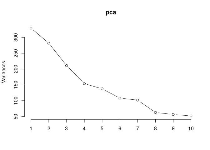
summary(pca)## Importance of components:
## PC1 PC2 PC3 PC4 PC5 PC6
## Standard deviation 18.1536 16.7875 14.5261 12.40665 11.7212 10.39141
## Proportion of Variance 0.1941 0.1659 0.1242 0.09064 0.0809 0.06358
## Cumulative Proportion 0.1941 0.3600 0.4843 0.57490 0.6558 0.71938
## PC7 PC8 PC9 PC10 PC11 PC12 PC13
## Standard deviation 10.08458 7.91536 7.50449 7.19448 7.02543 6.49725 6.31882
## Proportion of Variance 0.05989 0.03689 0.03316 0.03048 0.02906 0.02486 0.02351
## Cumulative Proportion 0.77927 0.81616 0.84932 0.87980 0.90887 0.93372 0.95723
## PC14 PC15 PC16
## Standard deviation 6.08628 5.96516 1.65e-14
## Proportion of Variance 0.02181 0.02095 0.00e+00
## Cumulative Proportion 0.97905 1.00000 1.00e+00Treatment_time_color <- as.factor(tdata.FPKM.sample.info.small.intestine$treatment_time)
Treatment_time_color <- as.data.frame(Treatment_time_color)
col_treatment_time <- colorRampPalette(brewer.pal(n = 12, name = "Paired"))(4)[Treatment_time_color$Treatment_time_color]
pca_treatment_time <- cbind(Treatment_time_color,pca$x[,1],pca$x[,2])
pca_treatment_time <- as.data.frame(pca_treatment_time)
p <- ggplot(pca_treatment_time,aes(pca$x[,1], pca$x[,2]))
p <- p + geom_point(aes(fill = as.factor(pca_treatment_time$Treatment_time_color)), shape=21, size=4) + theme_bw()
p <- p + theme(legend.title = element_text(size=10,face="bold")) +
theme(legend.text = element_text(size=10, face="bold"))
p <- p + xlab("PCA 1 (19.41%)") + ylab("PCA 2 (16.59%)") + theme(axis.title = element_text(face="bold"))
p <- p + stat_ellipse(aes(pca$x[,1], pca$x[,2], group = Treatment_time_color, fill = as.factor(pca_treatment_time$Treatment_time_color)), geom="polygon",level=0.95,alpha=0.4) +
scale_fill_manual(values=c("#ED8F47", "#B89B74", "#A6CEE3", "#B15928"),name="Treatment Type and Time",
breaks=c("None 4 wks", "2DG 96 hrs", "2DG 4 wks", "None 96 hrs"),
labels=c("None 4 wks", "2DG 96 hrs", "2DG 4 wks", "None 96 hrs")) +
scale_linetype_manual(values=c(1,2))
print(p)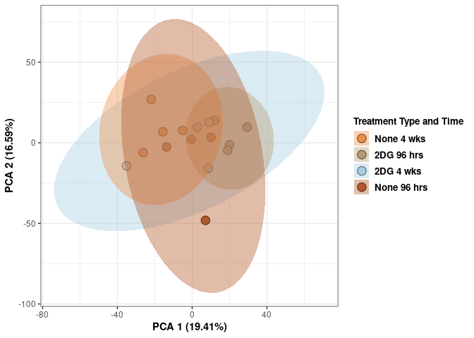
Treatment small intestine
Treatment_color <- as.factor(tdata.FPKM.sample.info.small.intestine$Treatment)
Treatment_color <- as.data.frame(Treatment_color)
col_treatment <- colorRampPalette(brewer.pal(n = 12, name = "Paired"))(2)[Treatment_color$Treatment_color]
pca_treatment <- cbind(Treatment_color,pca$x[,1],pca$x[,2])
pca_treatment <- as.data.frame(pca_treatment)

p <- ggplot(pca_treatment,aes(pca$x[,1], pca$x[,2]))
p <- p + geom_point(aes(fill = as.factor(pca_treatment$Treatment_color)), shape=21, size=4) + theme_bw()
p <- p + theme(legend.title = element_text(size=10,face="bold")) +
  theme(legend.text = element_text(size=10, face="bold"))
p <- p + xlab("PCA 1 (19.41%)") + ylab("PCA 2 (16.59%)") + theme(axis.title = element_text(face="bold"))
p <- p + stat_ellipse(aes(pca$x[,1], pca$x[,2], group = Treatment_color, fill = as.factor(pca_treatment$Treatment_color)), geom="polygon",level=0.95,alpha=0.4) +
  scale_fill_manual(values=c("#A6CEE3", "#B15928"),name="Treatment Type",
                       breaks=c("2DG", "None"),
                       labels=c("2DG", "small.intestine")) +
  scale_linetype_manual(values=c(1,2))
print(p)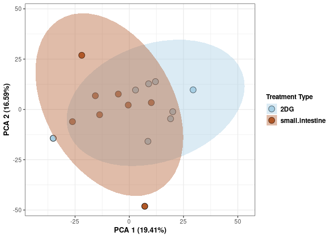
Time small intestine
Time_color <- as.factor(tdata.FPKM.sample.info.small.intestine$Time)
Time_color <- as.data.frame(Time_color)
col_time <- colorRampPalette(brewer.pal(n = 12, name = "Paired"))(2)[Time_color$Time_color]
pca_time <- cbind(Time_color,pca$x[,1],pca$x[,2])
pca_time <- as.data.frame(pca_time)

p <- ggplot(pca_time,aes(pca$x[,1], pca$x[,2]))
p <- p + geom_point(aes(fill = as.factor(pca_time$Time_color)), shape=21, size=4) + theme_bw()
p <- p + theme(legend.title = element_text(size=10,face="bold")) +
  theme(legend.text = element_text(size=10, face="bold"))
p <- p + xlab("PCA 1 (19.41%)") + ylab("PCA 2 (16.59%)") + theme(axis.title = element_text(face="bold"))
p <- p + stat_ellipse(aes(pca$x[,1], pca$x[,2], group = Time_color, fill = as.factor(pca_time$Time_color)), geom="polygon",level=0.95,alpha=0.4) +
  scale_fill_manual(values=c("#A6CEE3", "#B15928"),name="Time",
                       breaks=c("4 wks", "96 hrs"),
                       labels=c("4 wks", "96 hrs")) +
  scale_linetype_manual(values=c(1,2))
print(p)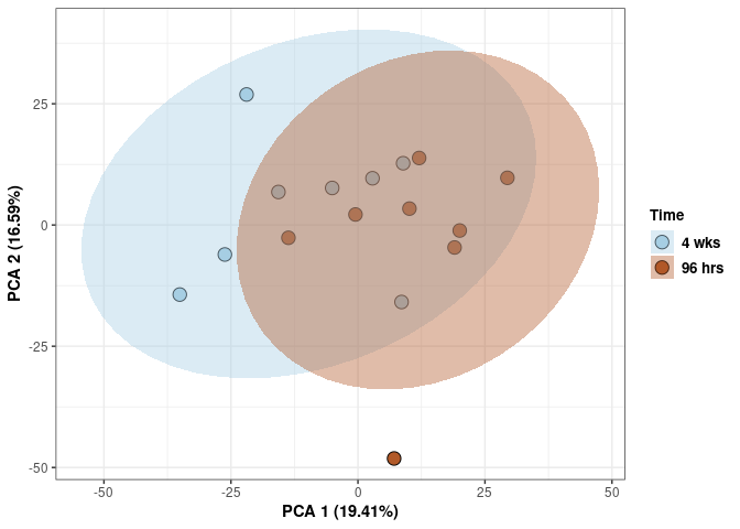
3D small intestine
This plot is color coded by time and treatment for small intestine, first collectively and then separately. To see each one click the names on the legend to make them disappear and click again to make them reappear.
Treatment_time_color <- as.factor(tdata.FPKM.sample.info.small.intestine$treatment_time)
Treatment_time_color <- as.data.frame(Treatment_time_color)
col_treatment_time <- colorRampPalette(brewer.pal(n = 12, name = "Paired"))(4)[Treatment_time_color$Treatment_time_color]
pca_treatment_time <- cbind(Treatment_time_color,pca$x[,1],pca$x[,2],pca$x[,3])
pca_treatment_time <- as.data.frame(pca_treatment_time)
rownames(pca_treatment_time) <- rownames(tdata.FPKM.sample.info.small.intestine)

p <- plot_ly(pca_treatment_time, x = pca_treatment_time$`pca$x[, 1]`, y = pca_treatment_time$`pca$x[, 2]`, z = pca_treatment_time$`pca$x[, 3]`, color = pca_treatment_time$Treatment_time_color, colors = c("#ED8F47", "#B89B74", "#A6CEE3", "#B15928"), text = rownames(pca_treatment_time)) %>%
  add_markers() %>%
  layout(scene = list(xaxis = list(title = "PC 1 19.42%"),
                     yaxis = list(title = "PC 2 16.59%"),
                     zaxis = list(title = "PC 3 12.42%")))

Treatment_color <- as.factor(tdata.FPKM.sample.info.small.intestine$Treatment)
Treatment_color <- as.data.frame(Treatment_color)
col_treatment <- colorRampPalette(brewer.pal(n = 12, name = "Paired"))(2)[Treatment_color$Treatment_color]
pca_treatment <- cbind(Treatment_color,pca$x[,1],pca$x[,2],pca$x[,3])
pca_treatment <- as.data.frame(pca_treatment)
rownames(pca_treatment) <- rownames(tdata.FPKM.sample.info.small.intestine)

p1 <- plot_ly(pca_treatment, x = pca_treatment$`pca$x[, 1]`, y = pca_treatment$`pca$x[, 2]`, z = pca_treatment$`pca$x[, 3]`, color = pca_treatment$Treatment_color, colors = c("#CC0000", "#330033"), text = rownames(pca_treatment)) %>%
  add_markers() %>%
  layout(scene = list(xaxis = list(title = "PC 1 19.41%"),
                     yaxis = list(title = "PC 2 16.59%"),
                     zaxis = list(title = "PC 3 12.42%")))

Time_color <- as.factor(tdata.FPKM.sample.info.small.intestine$Time)
Time_color <- as.data.frame(Time_color)
col_time <- colorRampPalette(brewer.pal(n = 12, name = "Paired"))(2)[Time_color$Time_color]
pca_time <- cbind(Time_color,pca$x[,1],pca$x[,2],pca$x[,3])
pca_time <- as.data.frame(pca_time)
rownames(pca_time) <- rownames(tdata.FPKM.sample.info.small.intestine)

p2 <- plot_ly(pca_time, x = pca_time$`pca$x[, 1]`, y = pca_time$`pca$x[, 2]`, z = pca_time$`pca$x[, 3]`, color = pca_time$Time_color, colors = c("#B8860B", "#00FA9A"), text = rownames(pca_time)) %>%
  add_markers() %>%
  layout(scene = list(xaxis = list(title = "PC 1 19.41%"),
                     yaxis = list(title = "PC 2 16.59%"),
                     zaxis = list(title = "PC 3 12.42%")))
p3 <- plotly::subplot(p,p1,p2)
p3
Scree plot and summary statistics skeletal muscle
tdata.FPKM.sample.info <- readRDS(here("Data","20190406_RNAseq_B6_4wk_2DG_counts_phenotypes.RData"))

tdata.FPKM.sample.info.skeletal.muscle <- rownames_to_column(tdata.FPKM.sample.info) %>% filter(Tissue=="Skeletal Muscle") %>% column_to_rownames('rowname')

tdata.FPKM <- readRDS(here("Data","20190406_RNAseq_B6_4wk_2DG_counts_numeric.RData"))

log.tdata.FPKM <- log(tdata.FPKM + 1)
log.tdata.FPKM <- as.data.frame(log.tdata.FPKM)

rows <- rownames(tdata.FPKM.sample.info.skeletal.muscle)

log.tdata.FPKM.skeletal.muscle <- rownames_to_column(log.tdata.FPKM)

log.tdata.FPKM.skeletal.muscle <- log.tdata.FPKM.skeletal.muscle %>% filter(rowname %in% rows) %>% column_to_rownames('rowname')

pca <- prcomp(log.tdata.FPKM.skeletal.muscle, center = T)

screeplot(pca,type = "lines")
summary(pca)## Importance of components:
## PC1 PC2 PC3 PC4 PC5 PC6
## Standard deviation 27.1777 15.4336 12.73250 11.47359 10.2621 9.28652
## Proportion of Variance 0.4012 0.1294 0.08806 0.07151 0.0572 0.04684
## Cumulative Proportion 0.4012 0.5306 0.61865 0.69015 0.7473 0.79420
## PC7 PC8 PC9 PC10 PC11 PC12 PC13
## Standard deviation 8.36152 7.43979 7.03602 6.76852 6.20206 5.95616 5.7252
## Proportion of Variance 0.03798 0.03007 0.02689 0.02488 0.02089 0.01927 0.0178
## Cumulative Proportion 0.83217 0.86224 0.88913 0.91401 0.93491 0.95418 0.9720
## PC14 PC15 PC16
## Standard deviation 5.22861 4.92414 1.304e-14
## Proportion of Variance 0.01485 0.01317 0.000e+00
## Cumulative Proportion 0.98683 1.00000 1.000e+00Treatment and time skeletal muscle
tdata.FPKM.sample.info <- readRDS(here("Data","20190406_RNAseq_B6_4wk_2DG_counts_phenotypes.RData"))

treatment_time <-paste(tdata.FPKM.sample.info$Treatment, tdata.FPKM.sample.info$Time)

tdata.FPKM.sample.info <-cbind(tdata.FPKM.sample.info,treatment_time)

tdata.FPKM.sample.info.skeletal.muscle <- rownames_to_column(tdata.FPKM.sample.info) %>% filter(Tissue=="Skeletal Muscle") %>% column_to_rownames('rowname')

tdata.FPKM <- readRDS(here("Data","20190406_RNAseq_B6_4wk_2DG_counts_numeric.RData"))

log.tdata.FPKM <- log(tdata.FPKM + 1)
log.tdata.FPKM <- as.data.frame(log.tdata.FPKM)

rows <- rownames(tdata.FPKM.sample.info.skeletal.muscle)

log.tdata.FPKM.skeletal.muscle <- rownames_to_column(log.tdata.FPKM)

log.tdata.FPKM.skeletal.muscle <- log.tdata.FPKM.skeletal.muscle %>% filter(rowname %in% rows) %>% column_to_rownames('rowname')

pca <- prcomp(log.tdata.FPKM.skeletal.muscle, center = T)

screeplot(pca,type = "lines")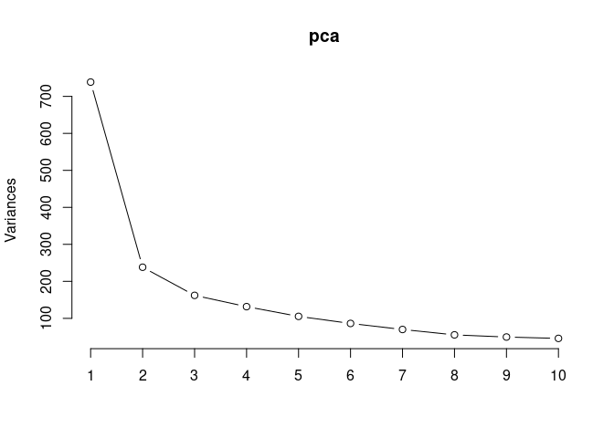
summary(pca)## Importance of components:
## PC1 PC2 PC3 PC4 PC5 PC6
## Standard deviation 27.1777 15.4336 12.73250 11.47359 10.2621 9.28652
## Proportion of Variance 0.4012 0.1294 0.08806 0.07151 0.0572 0.04684
## Cumulative Proportion 0.4012 0.5306 0.61865 0.69015 0.7473 0.79420
## PC7 PC8 PC9 PC10 PC11 PC12 PC13
## Standard deviation 8.36152 7.43979 7.03602 6.76852 6.20206 5.95616 5.7252
## Proportion of Variance 0.03798 0.03007 0.02689 0.02488 0.02089 0.01927 0.0178
## Cumulative Proportion 0.83217 0.86224 0.88913 0.91401 0.93491 0.95418 0.9720
## PC14 PC15 PC16
## Standard deviation 5.22861 4.92414 1.304e-14
## Proportion of Variance 0.01485 0.01317 0.000e+00
## Cumulative Proportion 0.98683 1.00000 1.000e+00Treatment_time_color <- as.factor(tdata.FPKM.sample.info.skeletal.muscle$treatment_time)
Treatment_time_color <- as.data.frame(Treatment_time_color)
col_treatment_time <- colorRampPalette(brewer.pal(n = 12, name = "Paired"))(4)[Treatment_time_color$Treatment_time_color]
pca_treatment_time <- cbind(Treatment_time_color,pca$x[,1],pca$x[,2])
pca_treatment_time <- as.data.frame(pca_treatment_time)
p <- ggplot(pca_treatment_time,aes(pca$x[,1], pca$x[,2]))
p <- p + geom_point(aes(fill = as.factor(pca_treatment_time$Treatment_time_color)), shape=21, size=4) + theme_bw()
p <- p + theme(legend.title = element_text(size=10,face="bold")) +
theme(legend.text = element_text(size=10, face="bold"))
p <- p + xlab("PCA 1 (40.12%)") + ylab("PCA 2 (12.94%)") + theme(axis.title = element_text(face="bold"))
p <- p + stat_ellipse(aes(pca$x[,1], pca$x[,2], group = Treatment_time_color, fill = as.factor(pca_treatment_time$Treatment_time_color)), geom="polygon",level=0.95,alpha=0.4) +
scale_fill_manual(values=c("#ED8F47", "#B89B74", "#A6CEE3", "#B15928"),name="Treatment Type and Time",
breaks=c("None 4 wks", "2DG 96 hrs", "2DG 4 wks", "None 96 hrs"),
labels=c("None 4 wks", "2DG 96 hrs", "2DG 4 wks", "None 96 hrs")) +
scale_linetype_manual(values=c(1,2))
print(p)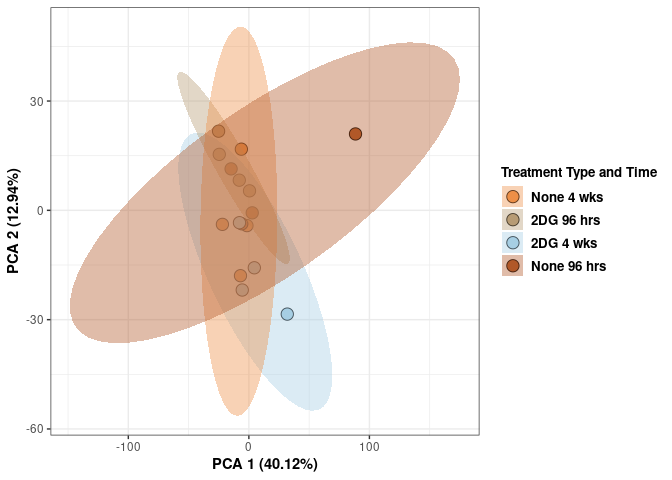
Treatment skeletal muscle
Treatment_color <- as.factor(tdata.FPKM.sample.info.skeletal.muscle$Treatment)
Treatment_color <- as.data.frame(Treatment_color)
col_treatment <- colorRampPalette(brewer.pal(n = 12, name = "Paired"))(2)[Treatment_color$Treatment_color]
pca_treatment <- cbind(Treatment_color,pca$x[,1],pca$x[,2])
pca_treatment <- as.data.frame(pca_treatment)

p <- ggplot(pca_treatment,aes(pca$x[,1], pca$x[,2]))
p <- p + geom_point(aes(fill = as.factor(pca_treatment$Treatment_color)), shape=21, size=4) + theme_bw()
p <- p + theme(legend.title = element_text(size=10,face="bold")) +
  theme(legend.text = element_text(size=10, face="bold"))
p <- p + xlab("PCA 1 (40.12%)") + ylab("PCA 2 (12.94%)") + theme(axis.title = element_text(face="bold"))
p <- p + stat_ellipse(aes(pca$x[,1], pca$x[,2], group = Treatment_color, fill = as.factor(pca_treatment$Treatment_color)), geom="polygon",level=0.95,alpha=0.4) +
  scale_fill_manual(values=c("#A6CEE3", "#B15928"),name="Treatment Type",
                       breaks=c("2DG", "None"),
                       labels=c("2DG", "skeletal.muscle")) +
  scale_linetype_manual(values=c(1,2))
print(p)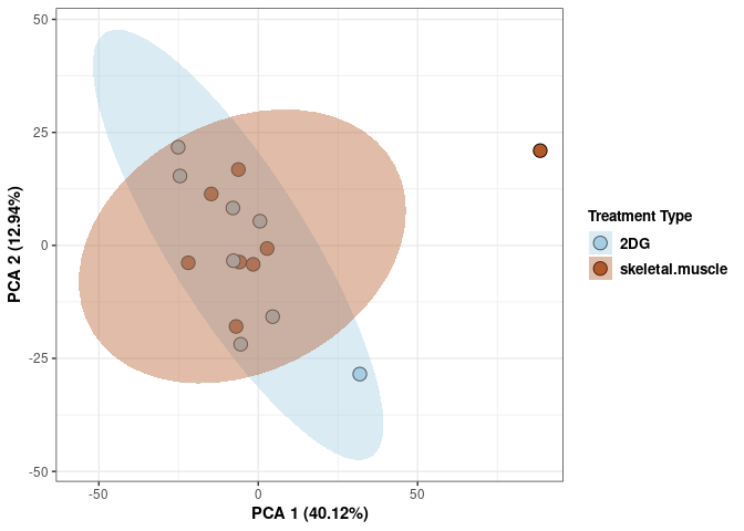
##Time skeletal muscle
Time_color <- as.factor(tdata.FPKM.sample.info.skeletal.muscle$Time)
Time_color <- as.data.frame(Time_color)
col_time <- colorRampPalette(brewer.pal(n = 12, name = "Paired"))(2)[Time_color$Time_color]
pca_time <- cbind(Time_color,pca$x[,1],pca$x[,2])
pca_time <- as.data.frame(pca_time)

p <- ggplot(pca_time,aes(pca$x[,1], pca$x[,2]))
p <- p + geom_point(aes(fill = as.factor(pca_time$Time_color)), shape=21, size=4) + theme_bw()
p <- p + theme(legend.title = element_text(size=10,face="bold")) +
  theme(legend.text = element_text(size=10, face="bold"))
p <- p + xlab("PCA 1 (40.12%)") + ylab("PCA 2 (12.94%)") + theme(axis.title = element_text(face="bold"))
p <- p + stat_ellipse(aes(pca$x[,1], pca$x[,2], group = Time_color, fill = as.factor(pca_time$Time_color)), geom="polygon",level=0.95,alpha=0.4) +
  scale_fill_manual(values=c("#A6CEE3", "#B15928"),name="Time",
                       breaks=c("4 wks", "96 hrs"),
                       labels=c("4 wks", "96 hrs")) +
  scale_linetype_manual(values=c(1,2))
print(p)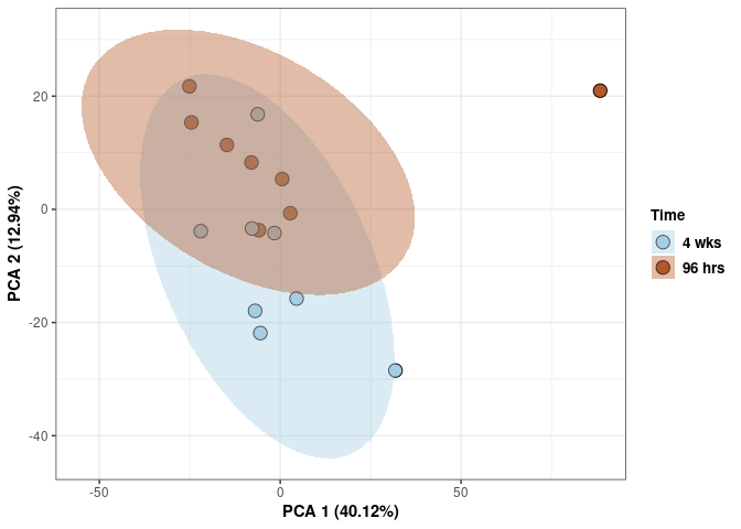
3D skeletal muscle
This plot is color coded by time and treatment for skeletal muscle, first collectively and then separately. To see each one click the names on the legend to make them disappear and click again to make them reappear.
Treatment_time_color <- as.factor(tdata.FPKM.sample.info.skeletal.muscle$treatment_time)
Treatment_time_color <- as.data.frame(Treatment_time_color)
col_treatment_time <- colorRampPalette(brewer.pal(n = 12, name = "Paired"))(4)[Treatment_time_color$Treatment_time_color]
pca_treatment_time <- cbind(Treatment_time_color,pca$x[,1],pca$x[,2],pca$x[,3])
pca_treatment_time <- as.data.frame(pca_treatment_time)
rownames(pca_treatment_time) <- rownames(tdata.FPKM.sample.info.skeletal.muscle)

p <- plot_ly(pca_treatment_time, x = pca_treatment_time$`pca$x[, 1]`, y = pca_treatment_time$`pca$x[, 2]`, z = pca_treatment_time$`pca$x[, 3]`, color = pca_treatment_time$Treatment_time_color, colors = c("#ED8F47", "#B89B74", "#A6CEE3", "#B15928"), text = rownames(pca_treatment_time)) %>%
  add_markers() %>%
  layout(scene = list(xaxis = list(title = "PC 1 40.12%"),
                     yaxis = list(title = "PC 2 12.94%"),
                     zaxis = list(title = "PC 3 8.81%")))

Treatment_color <- as.factor(tdata.FPKM.sample.info.skeletal.muscle$Treatment)
Treatment_color <- as.data.frame(Treatment_color)
col_treatment <- colorRampPalette(brewer.pal(n = 12, name = "Paired"))(2)[Treatment_color$Treatment_color]
pca_treatment <- cbind(Treatment_color,pca$x[,1],pca$x[,2],pca$x[,3])
pca_treatment <- as.data.frame(pca_treatment)
rownames(pca_treatment) <- rownames(tdata.FPKM.sample.info.skeletal.muscle)

p1 <- plot_ly(pca_treatment, x = pca_treatment$`pca$x[, 1]`, y = pca_treatment$`pca$x[, 2]`, z = pca_treatment$`pca$x[, 3]`, color = pca_treatment$Treatment_color, colors = c("#CC0000", "#330033"), text = rownames(pca_treatment)) %>%
  add_markers() %>%
  layout(scene = list(xaxis = list(title = "PC 1 40.12%"),
                     yaxis = list(title = "PC 2 12.94%"),
                     zaxis = list(title = "PC 3 8.81%")))

Time_color <- as.factor(tdata.FPKM.sample.info.skeletal.muscle$Time)
Time_color <- as.data.frame(Time_color)
col_time <- colorRampPalette(brewer.pal(n = 12, name = "Paired"))(2)[Time_color$Time_color]
pca_time <- cbind(Time_color,pca$x[,1],pca$x[,2],pca$x[,3])
pca_time <- as.data.frame(pca_time)
rownames(pca_time) <- rownames(tdata.FPKM.sample.info.skeletal.muscle)

p2 <- plot_ly(pca_time, x = pca_time$`pca$x[, 1]`, y = pca_time$`pca$x[, 2]`, z = pca_time$`pca$x[, 3]`, color = pca_time$Time_color, colors = c("#B8860B", "#00FA9A"), text = rownames(pca_time)) %>%
  add_markers() %>%
  layout(scene = list(xaxis = list(title = "PC 1 40.12%"),
                     yaxis = list(title = "PC 2 12.94%"),
                     zaxis = list(title = "PC 3 8.81%")))
p3 <- plotly::subplot(p,p1,p2)
p3
Scree plot and summary statistics prefrontal cortex
tdata.FPKM.sample.info <- readRDS(here("Data","20190406_RNAseq_B6_4wk_2DG_counts_phenotypes.RData"))

tdata.FPKM.sample.info.prefrontal.cortex <- rownames_to_column(tdata.FPKM.sample.info) %>% filter(Tissue=="Pre-frontal Cortex") %>% column_to_rownames('rowname')

tdata.FPKM <- readRDS(here("Data","20190406_RNAseq_B6_4wk_2DG_counts_numeric.RData"))

log.tdata.FPKM <- log(tdata.FPKM + 1)
log.tdata.FPKM <- as.data.frame(log.tdata.FPKM)

rows <- rownames(tdata.FPKM.sample.info.prefrontal.cortex)

log.tdata.FPKM.prefrontal.cortex <- rownames_to_column(log.tdata.FPKM)

log.tdata.FPKM.prefrontal.cortex <- log.tdata.FPKM.prefrontal.cortex %>% filter(rowname %in% rows) %>% column_to_rownames('rowname')

pca <- prcomp(log.tdata.FPKM.prefrontal.cortex, center = T)

screeplot(pca,type = "lines")
summary(pca)## Importance of components:
## PC1 PC2 PC3 PC4 PC5 PC6 PC7
## Standard deviation 18.065 14.7905 12.4111 10.79428 9.6095 7.12852 6.37461
## Proportion of Variance 0.264 0.1770 0.1246 0.09425 0.0747 0.04111 0.03287
## Cumulative Proportion 0.264 0.4409 0.5655 0.65980 0.7345 0.77560 0.80847
## PC8 PC9 PC10 PC11 PC12 PC13 PC14
## Standard deviation 5.96477 5.89062 5.70641 5.47843 5.30616 5.22067 5.11748
## Proportion of Variance 0.02878 0.02807 0.02634 0.02428 0.02278 0.02205 0.02118
## Cumulative Proportion 0.83725 0.86532 0.89166 0.91594 0.93871 0.96076 0.98195
## PC15 PC16
## Standard deviation 4.72422 1.626e-14
## Proportion of Variance 0.01805 0.000e+00
## Cumulative Proportion 1.00000 1.000e+00Treatment and time prefrontal cortex
tdata.FPKM.sample.info <- readRDS(here("Data","20190406_RNAseq_B6_4wk_2DG_counts_phenotypes.RData"))

treatment_time <-paste(tdata.FPKM.sample.info$Treatment, tdata.FPKM.sample.info$Time)

tdata.FPKM.sample.info <-cbind(tdata.FPKM.sample.info,treatment_time)

tdata.FPKM.sample.info.prefrontal.cortex <- rownames_to_column(tdata.FPKM.sample.info) %>% filter(Tissue=="Pre-frontal Cortex") %>% column_to_rownames('rowname')

tdata.FPKM <- readRDS(here("Data","20190406_RNAseq_B6_4wk_2DG_counts_numeric.RData"))

log.tdata.FPKM <- log(tdata.FPKM + 1)
log.tdata.FPKM <- as.data.frame(log.tdata.FPKM)

rows <- rownames(tdata.FPKM.sample.info.prefrontal.cortex)

log.tdata.FPKM.prefrontal.cortex <- rownames_to_column(log.tdata.FPKM)

log.tdata.FPKM.prefrontal.cortex <- log.tdata.FPKM.prefrontal.cortex %>% filter(rowname %in% rows) %>% column_to_rownames('rowname')

pca <- prcomp(log.tdata.FPKM.prefrontal.cortex, center = T)

screeplot(pca,type = "lines")
summary(pca)## Importance of components:
## PC1 PC2 PC3 PC4 PC5 PC6 PC7
## Standard deviation 18.065 14.7905 12.4111 10.79428 9.6095 7.12852 6.37461
## Proportion of Variance 0.264 0.1770 0.1246 0.09425 0.0747 0.04111 0.03287
## Cumulative Proportion 0.264 0.4409 0.5655 0.65980 0.7345 0.77560 0.80847
## PC8 PC9 PC10 PC11 PC12 PC13 PC14
## Standard deviation 5.96477 5.89062 5.70641 5.47843 5.30616 5.22067 5.11748
## Proportion of Variance 0.02878 0.02807 0.02634 0.02428 0.02278 0.02205 0.02118
## Cumulative Proportion 0.83725 0.86532 0.89166 0.91594 0.93871 0.96076 0.98195
## PC15 PC16
## Standard deviation 4.72422 1.626e-14
## Proportion of Variance 0.01805 0.000e+00
## Cumulative Proportion 1.00000 1.000e+00Treatment_time_color <- as.factor(tdata.FPKM.sample.info.prefrontal.cortex$treatment_time)
Treatment_time_color <- as.data.frame(Treatment_time_color)
col_treatment_time <- colorRampPalette(brewer.pal(n = 12, name = "Paired"))(4)[Treatment_time_color$Treatment_time_color]
pca_treatment_time <- cbind(Treatment_time_color,pca$x[,1],pca$x[,2])
pca_treatment_time <- as.data.frame(pca_treatment_time)
p <- ggplot(pca_treatment_time,aes(pca$x[,1], pca$x[,2]))
p <- p + geom_point(aes(fill = as.factor(pca_treatment_time$Treatment_time_color)), shape=21, size=4) + theme_bw()
p <- p + theme(legend.title = element_text(size=10,face="bold")) +
theme(legend.text = element_text(size=10, face="bold"))
p <- p + xlab("PCA 1 (26.4%)") + ylab("PCA 2 (17.7%)") + theme(axis.title = element_text(face="bold"))
p <- p + stat_ellipse(aes(pca$x[,1], pca$x[,2], group = Treatment_time_color, fill = as.factor(pca_treatment_time$Treatment_time_color)), geom="polygon",level=0.95,alpha=0.4) +
scale_fill_manual(values=c("#ED8F47", "#B89B74", "#A6CEE3", "#B15928"),name="Treatment Type and Time",
breaks=c("None 4 wks", "2DG 96 hrs", "2DG 4 wks", "None 96 hrs"),
labels=c("None 4 wks", "2DG 96 hrs", "2DG 4 wks", "None 96 hrs")) +
scale_linetype_manual(values=c(1,2))
print(p)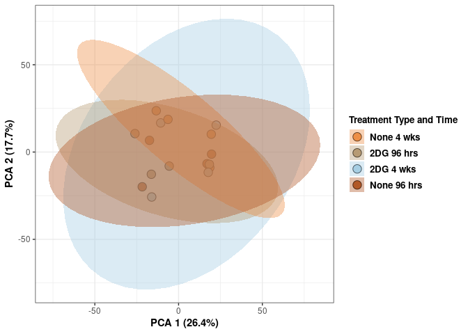
Treatment prefrontal cortex
Treatment_color <- as.factor(tdata.FPKM.sample.info.prefrontal.cortex$Treatment)
Treatment_color <- as.data.frame(Treatment_color)
col_treatment <- colorRampPalette(brewer.pal(n = 12, name = "Paired"))(2)[Treatment_color$Treatment_color]
pca_treatment <- cbind(Treatment_color,pca$x[,1],pca$x[,2])
pca_treatment <- as.data.frame(pca_treatment)

p <- ggplot(pca_treatment,aes(pca$x[,1], pca$x[,2]))
p <- p + geom_point(aes(fill = as.factor(pca_treatment$Treatment_color)), shape=21, size=4) + theme_bw()
p <- p + theme(legend.title = element_text(size=10,face="bold")) +
  theme(legend.text = element_text(size=10, face="bold"))
p <- p + xlab("PCA 1 (26.4%)") + ylab("PCA 2 (17.7%)") + theme(axis.title = element_text(face="bold"))
p <- p + stat_ellipse(aes(pca$x[,1], pca$x[,2], group = Treatment_color, fill = as.factor(pca_treatment$Treatment_color)), geom="polygon",level=0.95,alpha=0.4) +
  scale_fill_manual(values=c("#A6CEE3", "#B15928"),name="Treatment Type",
                       breaks=c("2DG", "None"),
                       labels=c("2DG", "prefrontal.cortex")) +
  scale_linetype_manual(values=c(1,2))
print(p)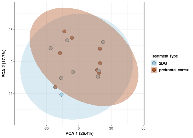
Time prefrontal cortex
Time_color <- as.factor(tdata.FPKM.sample.info.prefrontal.cortex$Time)
Time_color <- as.data.frame(Time_color)
col_time <- colorRampPalette(brewer.pal(n = 12, name = "Paired"))(2)[Time_color$Time_color]
pca_time <- cbind(Time_color,pca$x[,1],pca$x[,2])
pca_time <- as.data.frame(pca_time)

p <- ggplot(pca_time,aes(pca$x[,1], pca$x[,2]))
p <- p + geom_point(aes(fill = as.factor(pca_time$Time_color)), shape=21, size=4) + theme_bw()
p <- p + theme(legend.title = element_text(size=10,face="bold")) +
  theme(legend.text = element_text(size=10, face="bold"))
p <- p + xlab("PCA 1 (26.4%)") + ylab("PCA 2 (17.7%)") + theme(axis.title = element_text(face="bold"))
p <- p + stat_ellipse(aes(pca$x[,1], pca$x[,2], group = Time_color, fill = as.factor(pca_time$Time_color)), geom="polygon",level=0.95,alpha=0.4) +
  scale_fill_manual(values=c("#A6CEE3", "#B15928"),name="Time",
                       breaks=c("4 wks", "96 hrs"),
                       labels=c("4 wks", "96 hrs")) +
  scale_linetype_manual(values=c(1,2))
print(p)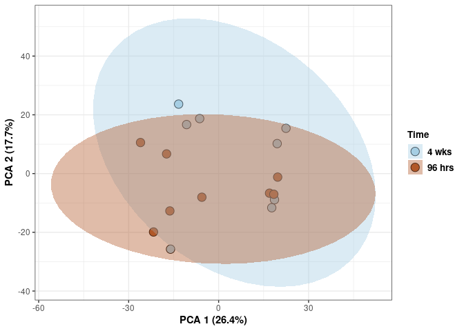
3D pre-frontal cortex
This plot is color coded by time and treatment for pre-frontal cortex, first collectively and then separately. To see each one click the names on the legend to make them disappear and click again to make them reappear.
Treatment_time_color <- as.factor(tdata.FPKM.sample.info.prefrontal.cortex$treatment_time)
Treatment_time_color <- as.data.frame(Treatment_time_color)
col_treatment_time <- colorRampPalette(brewer.pal(n = 12, name = "Paired"))(4)[Treatment_time_color$Treatment_time_color]
pca_treatment_time <- cbind(Treatment_time_color,pca$x[,1],pca$x[,2],pca$x[,3])
pca_treatment_time <- as.data.frame(pca_treatment_time)
rownames(pca_treatment_time) <- rownames(tdata.FPKM.sample.info.prefrontal.cortex)

p <- plot_ly(pca_treatment_time, x = pca_treatment_time$`pca$x[, 1]`, y = pca_treatment_time$`pca$x[, 2]`, z = pca_treatment_time$`pca$x[, 3]`, color = pca_treatment_time$Treatment_time_color, colors = c("#ED8F47", "#B89B74", "#A6CEE3", "#B15928"), text = rownames(pca_treatment_time)) %>%
  add_markers() %>%
  layout(scene = list(xaxis = list(title = "PC 1 26.4%"),
                     yaxis = list(title = "PC 2 17.7%"),
                     zaxis = list(title = "PC 3 12.46%")))

Treatment_color <- as.factor(tdata.FPKM.sample.info.prefrontal.cortex$Treatment)
Treatment_color <- as.data.frame(Treatment_color)
col_treatment <- colorRampPalette(brewer.pal(n = 12, name = "Paired"))(2)[Treatment_color$Treatment_color]
pca_treatment <- cbind(Treatment_color,pca$x[,1],pca$x[,2],pca$x[,3])
pca_treatment <- as.data.frame(pca_treatment)
rownames(pca_treatment) <- rownames(tdata.FPKM.sample.info.prefrontal.cortex)

p1 <- plot_ly(pca_treatment, x = pca_treatment$`pca$x[, 1]`, y = pca_treatment$`pca$x[, 2]`, z = pca_treatment$`pca$x[, 3]`, color = pca_treatment$Treatment_color, colors = c("#CC0000", "#330033"), text = rownames(pca_treatment)) %>%
  add_markers() %>%
  layout(scene = list(xaxis = list(title = "PC 1 26.4%"),
                     yaxis = list(title = "PC 2 17.7%"),
                     zaxis = list(title = "PC 3 12.46%")))

Time_color <- as.factor(tdata.FPKM.sample.info.prefrontal.cortex$Time)
Time_color <- as.data.frame(Time_color)
col_time <- colorRampPalette(brewer.pal(n = 12, name = "Paired"))(2)[Time_color$Time_color]
pca_time <- cbind(Time_color,pca$x[,1],pca$x[,2],pca$x[,3])
pca_time <- as.data.frame(pca_time)
rownames(pca_time) <- rownames(tdata.FPKM.sample.info.prefrontal.cortex)

p2 <- plot_ly(pca_time, x = pca_time$`pca$x[, 1]`, y = pca_time$`pca$x[, 2]`, z = pca_time$`pca$x[, 3]`, color = pca_time$Time_color, colors = c("#B8860B", "#00FA9A"), text = rownames(pca_time)) %>%
  add_markers() %>%
  layout(scene = list(xaxis = list(title = "PC 1 26.4%"),
                     yaxis = list(title = "PC 2 17.7%"),
                     zaxis = list(title = "PC 3 12.46%")))
p3 <- plotly::subplot(p,p1,p2)
p3
PCA (log Tissue 96hr 2DG)
These plots subset the data so each plot contains mice treated with 2DG for 96hrs for each tissue.
Scree plot and summary statistics
tdata.FPKM.sample.info <- readRDS(here("Data","20190406_RNAseq_B6_4wk_2DG_counts_phenotypes.RData"))

tdata.FPKM.sample.info.tissue.2DG.96hr <- rownames_to_column(tdata.FPKM.sample.info) %>% filter(Treatment=="2DG" & Time=="96 hrs") %>% column_to_rownames('rowname')

tdata.FPKM <- readRDS(here("Data","20190406_RNAseq_B6_4wk_2DG_counts_numeric.RData"))

log.tdata.FPKM <- log(tdata.FPKM + 1)
log.tdata.FPKM <- as.data.frame(log.tdata.FPKM)

rows <- rownames(tdata.FPKM.sample.info.tissue.2DG.96hr)

log.tdata.FPKM.tissue.2DG.96hr <- rownames_to_column(log.tdata.FPKM)

log.tdata.FPKM.tissue.2DG.96hr <- log.tdata.FPKM.tissue.2DG.96hr %>% filter(rowname %in% rows) %>% column_to_rownames('rowname')

pca <- prcomp(log.tdata.FPKM.tissue.2DG.96hr, center = T)

screeplot(pca,type = "lines")
summary(pca)## Importance of components:
## PC1 PC2 PC3 PC4 PC5 PC6
## Standard deviation 78.4069 56.5018 45.8883 39.6558 31.32181 21.72707
## Proportion of Variance 0.3973 0.2063 0.1361 0.1016 0.06341 0.03051
## Cumulative Proportion 0.3973 0.6037 0.7398 0.8414 0.90480 0.93531
## PC7 PC8 PC9 PC10 PC11 PC12
## Standard deviation 14.99984 11.64311 9.23067 8.97827 6.48065 5.94417
## Proportion of Variance 0.01454 0.00876 0.00551 0.00521 0.00271 0.00228
## Cumulative Proportion 0.94985 0.95861 0.96412 0.96933 0.97204 0.97432
## PC13 PC14 PC15 PC16 PC17 PC18 PC19
## Standard deviation 5.62913 5.47325 5.39044 5.20471 4.63557 4.53967 4.45051
## Proportion of Variance 0.00205 0.00194 0.00188 0.00175 0.00139 0.00133 0.00128
## Cumulative Proportion 0.97637 0.97831 0.98019 0.98194 0.98333 0.98466 0.98594
## PC20 PC21 PC22 PC23 PC24 PC25 PC26
## Standard deviation 4.3060 4.22103 4.08434 4.02850 3.90172 3.82368 3.74292
## Proportion of Variance 0.0012 0.00115 0.00108 0.00105 0.00098 0.00094 0.00091
## Cumulative Proportion 0.9871 0.98829 0.98937 0.99041 0.99140 0.99234 0.99325
## PC27 PC28 PC29 PC30 PC31 PC32 PC33
## Standard deviation 3.68685 3.65148 3.61101 3.5187 3.36707 3.33028 3.23264
## Proportion of Variance 0.00088 0.00086 0.00084 0.0008 0.00073 0.00072 0.00068
## Cumulative Proportion 0.99413 0.99499 0.99583 0.9966 0.99736 0.99808 0.99876
## PC34 PC35 PC36
## Standard deviation 3.14534 3.0556 3.482e-14
## Proportion of Variance 0.00064 0.0006 0.000e+00
## Cumulative Proportion 0.99940 1.0000 1.000e+00Tissue
Tissue_color <- as.factor(tdata.FPKM.sample.info.tissue.2DG.96hr$Tissue)
Tissue_color <- as.data.frame(Tissue_color)
col_tissue <- colorRampPalette(brewer.pal(n = 12, name = "Paired"))(9)[Tissue_color$Tissue_color]
pca_tissue <- cbind(Tissue_color,pca$x[,1],pca$x[,2])
pca_tissue <- as.data.frame(pca_tissue)

p <- ggplot(pca_tissue,aes(pca$x[,1], pca$x[,2]))
p <- p + geom_point(aes(fill = as.factor(pca_tissue$Tissue_color)), shape=21, size=4) + theme_bw()
p <- p + theme(legend.title = element_text(size=10,face="bold")) +
  theme(legend.text = element_text(size=10, face="bold"))
p <- p+ xlab("PCA 1 (39.73%)") + ylab("PCA 2 (20.63%)") + theme(axis.title = element_text(face="bold"))
p <- p + stat_ellipse(aes(pca$x[,1], pca$x[,2], group = Tissue_color, fill = as.factor(pca_tissue$Tissue_color)), geom="polygon",level=0.95,alpha=0.2) +
  scale_fill_manual(values=c("#B15928", "#F88A89", "#F06C45", "#A6CEE3", "#52AF43", "#FE870D", "#C7B699", "#569EA4","#B294C7"),name="Tissue Type",
                       breaks=c("Spleen", "Kidney","Liver","Heart","Hypothanamus","Pre-frontal Cortex","Small Intestine","Hippocampus","Skeletal Muscle"),
                       labels=c("Spleen", "kidney","Liver","Heart","Hypothalamus","Pre-frontal Cortex","Small Intestine","Hippocampus","Skeletal Muscle")) +
  scale_linetype_manual(values=c(1,2,1,2,1))
print(p)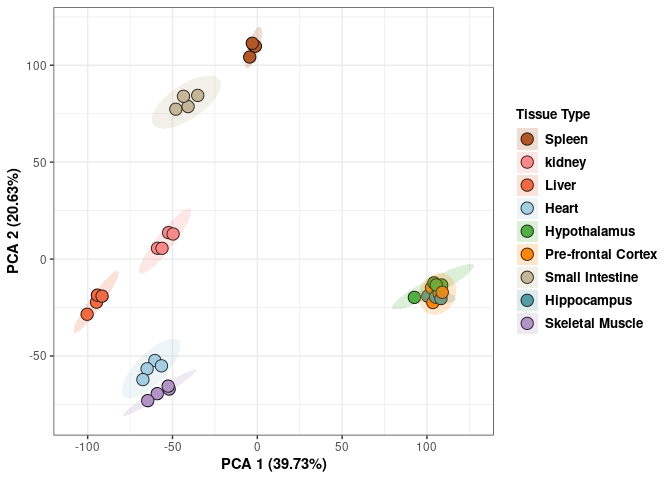
3D Tissue 2DG 96 hrs
Tissue_color <- as.factor(tdata.FPKM.sample.info.tissue.2DG.96hr$Tissue)
Tissue_color <- as.data.frame(Tissue_color)
col_tissue <- colorRampPalette(brewer.pal(n = 12, name = "Paired"))(9)[Tissue_color$Tissue_color]
pca_tissue <- cbind(Tissue_color,pca$x[,1],pca$x[,2],pca$x[,3])
pca_tissue <- as.data.frame(pca_tissue)
rownames(pca_tissue) <- rownames(tdata.FPKM.sample.info.tissue.2DG.96hr)

p <- plot_ly(pca_tissue, x = pca_tissue$`pca$x[, 1]`, y = pca_tissue$`pca$x[, 2]`, z = pca_tissue$`pca$x[, 3]`, color = pca_tissue$Tissue_color, colors = c("#B15928", "#F88A89", "#F06C45", "#A6CEE3", "#52AF43", "#FE870D", "#C7B699", "#569EA4","#B294C7"), text = rownames(pca_tissue)) %>%
  add_markers() %>%
  layout(scene = list(xaxis = list(title = "PC 1 39.73%"),
                     yaxis = list(title = "PC 2 20.63%"),
                     zaxis = list(title = "PC 3 13.61%")))
p
PCA (log Tissue 4wk 2DG)
Scree plot and summary statistics
tdata.FPKM.sample.info <- readRDS(here("Data","20190406_RNAseq_B6_4wk_2DG_counts_phenotypes.RData"))

tdata.FPKM.sample.info.tissue.2DG.4wk <- rownames_to_column(tdata.FPKM.sample.info) %>% filter(Treatment=="2DG" & Time=="4 wks") %>% column_to_rownames('rowname')

tdata.FPKM <- readRDS(here("Data","20190406_RNAseq_B6_4wk_2DG_counts_numeric.RData"))

log.tdata.FPKM <- log(tdata.FPKM + 1)
log.tdata.FPKM <- as.data.frame(log.tdata.FPKM)

rows <- rownames(tdata.FPKM.sample.info.tissue.2DG.4wk)

log.tdata.FPKM.tissue.2DG.4wk <- rownames_to_column(log.tdata.FPKM)

log.tdata.FPKM.tissue.2DG.4wk <- log.tdata.FPKM.tissue.2DG.4wk %>% filter(rowname %in% rows) %>% column_to_rownames('rowname')

pca <- prcomp(log.tdata.FPKM.tissue.2DG.4wk, center = T)

screeplot(pca,type = "lines")
summary(pca)## Importance of components:
## PC1 PC2 PC3 PC4 PC5 PC6
## Standard deviation 76.6999 53.7724 45.9234 38.50309 32.85504 19.48177
## Proportion of Variance 0.3914 0.1924 0.1403 0.09864 0.07183 0.02525
## Cumulative Proportion 0.3914 0.5838 0.7242 0.82280 0.89463 0.91988
## PC7 PC8 PC9 PC10 PC11 PC12 PC13
## Standard deviation 15.82730 14.38889 9.2556 8.44234 7.56305 6.90425 6.78081
## Proportion of Variance 0.01667 0.01378 0.0057 0.00474 0.00381 0.00317 0.00306
## Cumulative Proportion 0.93655 0.95033 0.9560 0.96077 0.96457 0.96775 0.97081
## PC14 PC15 PC16 PC17 PC18 PC19 PC20
## Standard deviation 6.6028 6.20732 5.6176 5.52721 5.13780 5.07961 4.92363
## Proportion of Variance 0.0029 0.00256 0.0021 0.00203 0.00176 0.00172 0.00161
## Cumulative Proportion 0.9737 0.97627 0.9784 0.98040 0.98216 0.98388 0.98549
## PC21 PC22 PC23 PC24 PC25 PC26 PC27
## Standard deviation 4.73690 4.26184 4.22560 4.15103 4.01372 3.88875 3.83605
## Proportion of Variance 0.00149 0.00121 0.00119 0.00115 0.00107 0.00101 0.00098
## Cumulative Proportion 0.98698 0.98819 0.98938 0.99053 0.99160 0.99260 0.99358
## PC28 PC29 PC30 PC31 PC32 PC33 PC34
## Standard deviation 3.75557 3.66397 3.58697 3.47925 3.45254 3.31852 3.26243
## Proportion of Variance 0.00094 0.00089 0.00086 0.00081 0.00079 0.00073 0.00071
## Cumulative Proportion 0.99452 0.99541 0.99627 0.99708 0.99787 0.99860 0.99931
## PC35 PC36
## Standard deviation 3.21974 3.406e-14
## Proportion of Variance 0.00069 0.000e+00
## Cumulative Proportion 1.00000 1.000e+00Tissue
Tissue_color <- as.factor(tdata.FPKM.sample.info.tissue.2DG.4wk$Tissue)
Tissue_color <- as.data.frame(Tissue_color)
col_tissue <- colorRampPalette(brewer.pal(n = 12, name = "Paired"))(9)[Tissue_color$Tissue_color]
pca_tissue <- cbind(Tissue_color,pca$x[,1],pca$x[,2])
pca_tissue <- as.data.frame(pca_tissue)

p <- ggplot(pca_tissue,aes(pca$x[,1], pca$x[,2]))
p <- p + geom_point(aes(fill = as.factor(pca_tissue$Tissue_color)), shape=21, size=4) + theme_bw()
p <- p + theme(legend.title = element_text(size=10,face="bold")) +
  theme(legend.text = element_text(size=10, face="bold"))
p <- p+ xlab("PCA 1 (39.14%)") + ylab("PCA 2 (19.24%)") + theme(axis.title = element_text(face="bold"))
p <- p + stat_ellipse(aes(pca$x[,1], pca$x[,2], group = Tissue_color, fill = as.factor(pca_tissue$Tissue_color)), geom="polygon",level=0.95,alpha=0.2) +
  scale_fill_manual(values=c("#B15928", "#F88A89", "#F06C45", "#A6CEE3", "#52AF43", "#FE870D", "#C7B699", "#569EA4","#B294C7"),name="Tissue Type",
                       breaks=c("Spleen", "Kidney","Liver","Heart","Hypothanamus","Pre-frontal Cortex","Small Intestine","Hippocampus","Skeletal Muscle"),
                       labels=c("Spleen", "kidney","Liver","Heart","Hypothalamus","Pre-frontal Cortex","Small Intestine","Hippocampus","Skeletal Muscle")) +
  scale_linetype_manual(values=c(1,2,1,2,1))
print(p)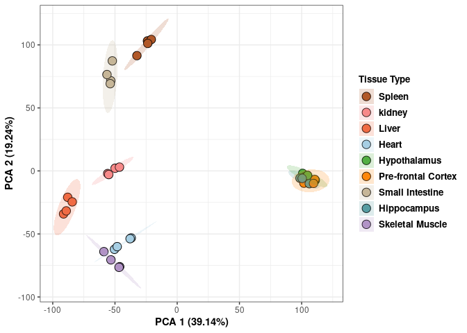
PCA (log Tissue 96hr control)
These plots subset the data so each plot contains mice treated with nothing for 96hrs for each tissue.
Scree plot and summary statistics
tdata.FPKM.sample.info <- readRDS(here("Data","20190406_RNAseq_B6_4wk_2DG_counts_phenotypes.RData"))

tdata.FPKM.sample.info.tissue.control.96hr <- rownames_to_column(tdata.FPKM.sample.info) %>% filter(Treatment=="None" & Time=="96 hrs") %>% column_to_rownames('rowname')

tdata.FPKM <- readRDS(here("Data","20190406_RNAseq_B6_4wk_2DG_counts_numeric.RData"))

log.tdata.FPKM <- log(tdata.FPKM + 1)
log.tdata.FPKM <- as.data.frame(log.tdata.FPKM)

rows <- rownames(tdata.FPKM.sample.info.tissue.control.96hr)

log.tdata.FPKM.tissue.control.96hr <- rownames_to_column(log.tdata.FPKM)

log.tdata.FPKM.tissue.control.96hr <- log.tdata.FPKM.tissue.control.96hr %>% filter(rowname %in% rows) %>% column_to_rownames('rowname')

pca <- prcomp(log.tdata.FPKM.tissue.control.96hr, center = T)

screeplot(pca,type = "lines")
summary(pca)## Importance of components:
## PC1 PC2 PC3 PC4 PC5 PC6
## Standard deviation 77.4486 56.4404 45.4801 37.64182 32.10891 19.46786
## Proportion of Variance 0.3906 0.2074 0.1347 0.09226 0.06713 0.02468
## Cumulative Proportion 0.3906 0.5980 0.7327 0.82490 0.89203 0.91671
## PC7 PC8 PC9 PC10 PC11 PC12
## Standard deviation 15.93035 14.35645 11.54847 8.9346 8.60300 7.41311
## Proportion of Variance 0.01652 0.01342 0.00868 0.0052 0.00482 0.00358
## Cumulative Proportion 0.93323 0.94665 0.95534 0.9605 0.96535 0.96893
## PC13 PC14 PC15 PC16 PC17 PC18 PC19
## Standard deviation 6.88598 6.59236 6.0767 5.89597 5.55159 5.12336 4.94489
## Proportion of Variance 0.00309 0.00283 0.0024 0.00226 0.00201 0.00171 0.00159
## Cumulative Proportion 0.97202 0.97485 0.9772 0.97951 0.98152 0.98323 0.98482
## PC20 PC21 PC22 PC23 PC24 PC25 PC26
## Standard deviation 4.87135 4.61828 4.2932 4.17821 4.02845 3.99551 3.89495
## Proportion of Variance 0.00155 0.00139 0.0012 0.00114 0.00106 0.00104 0.00099
## Cumulative Proportion 0.98637 0.98776 0.9890 0.99009 0.99115 0.99219 0.99318
## PC27 PC28 PC29 PC30 PC31 PC32 PC33
## Standard deviation 3.7186 3.65219 3.58312 3.5118 3.43526 3.31537 3.21589
## Proportion of Variance 0.0009 0.00087 0.00084 0.0008 0.00077 0.00072 0.00067
## Cumulative Proportion 0.9941 0.99495 0.99578 0.9966 0.99735 0.99807 0.99874
## PC34 PC35 PC36
## Standard deviation 3.17885 3.0346 3.439e-14
## Proportion of Variance 0.00066 0.0006 0.000e+00
## Cumulative Proportion 0.99940 1.0000 1.000e+00Tissue
Tissue_color <- as.factor(tdata.FPKM.sample.info.tissue.control.96hr$Tissue)
Tissue_color <- as.data.frame(Tissue_color)
col_tissue <- colorRampPalette(brewer.pal(n = 12, name = "Paired"))(9)[Tissue_color$Tissue_color]
pca_tissue <- cbind(Tissue_color,pca$x[,1],pca$x[,2])
pca_tissue <- as.data.frame(pca_tissue)

p <- ggplot(pca_tissue,aes(pca$x[,1], pca$x[,2]))
p <- p + geom_point(aes(fill = as.factor(pca_tissue$Tissue_color)), shape=21, size=4) + theme_bw()
p <- p + theme(legend.title = element_text(size=10,face="bold")) +
  theme(legend.text = element_text(size=10, face="bold"))
p <- p+ xlab("PCA 1 (39.06%)") + ylab("PCA 2 (20.74%)") + theme(axis.title = element_text(face="bold"))
p <- p + stat_ellipse(aes(pca$x[,1], pca$x[,2], group = Tissue_color, fill = as.factor(pca_tissue$Tissue_color)), geom="polygon",level=0.95,alpha=0.2) +
  scale_fill_manual(values=c("#B15928", "#F88A89", "#F06C45", "#A6CEE3", "#52AF43", "#FE870D", "#C7B699", "#569EA4","#B294C7"),name="Tissue Type",
                       breaks=c("Spleen", "Kidney","Liver","Heart","Hypothanamus","Pre-frontal Cortex","Small Intestine","Hippocampus","Skeletal Muscle"),
                       labels=c("Spleen", "kidney","Liver","Heart","Hypothalamus","Pre-frontal Cortex","Small Intestine","Hippocampus","Skeletal Muscle")) +
  scale_linetype_manual(values=c(1,2,1,2,1))
print(p)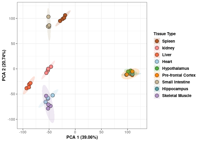
PCA (log Tissue 4wk 2DG)
These plots subset the data so each plot contains mice treated with 2DG for 4wks for each tissue.
Scree plot and summary statistics
tdata.FPKM.sample.info <- readRDS(here("Data","20190406_RNAseq_B6_4wk_2DG_counts_phenotypes.RData"))

tdata.FPKM.sample.info.tissue.2DG.4wk <- rownames_to_column(tdata.FPKM.sample.info) %>% filter(Treatment=="2DG" & Time=="4 wks") %>% column_to_rownames('rowname')

tdata.FPKM <- readRDS(here("Data","20190406_RNAseq_B6_4wk_2DG_counts_numeric.RData"))

log.tdata.FPKM <- log(tdata.FPKM + 1)
log.tdata.FPKM <- as.data.frame(log.tdata.FPKM)

rows <- rownames(tdata.FPKM.sample.info.tissue.2DG.4wk)

log.tdata.FPKM.tissue.2DG.4wk <- rownames_to_column(log.tdata.FPKM)

log.tdata.FPKM.tissue.2DG.4wk <- log.tdata.FPKM.tissue.2DG.4wk %>% filter(rowname %in% rows) %>% column_to_rownames('rowname')

pca <- prcomp(log.tdata.FPKM.tissue.2DG.4wk, center = T)

screeplot(pca,type = "lines")
summary(pca)## Importance of components:
## PC1 PC2 PC3 PC4 PC5 PC6
## Standard deviation 76.6999 53.7724 45.9234 38.50309 32.85504 19.48177
## Proportion of Variance 0.3914 0.1924 0.1403 0.09864 0.07183 0.02525
## Cumulative Proportion 0.3914 0.5838 0.7242 0.82280 0.89463 0.91988
## PC7 PC8 PC9 PC10 PC11 PC12 PC13
## Standard deviation 15.82730 14.38889 9.2556 8.44234 7.56305 6.90425 6.78081
## Proportion of Variance 0.01667 0.01378 0.0057 0.00474 0.00381 0.00317 0.00306
## Cumulative Proportion 0.93655 0.95033 0.9560 0.96077 0.96457 0.96775 0.97081
## PC14 PC15 PC16 PC17 PC18 PC19 PC20
## Standard deviation 6.6028 6.20732 5.6176 5.52721 5.13780 5.07961 4.92363
## Proportion of Variance 0.0029 0.00256 0.0021 0.00203 0.00176 0.00172 0.00161
## Cumulative Proportion 0.9737 0.97627 0.9784 0.98040 0.98216 0.98388 0.98549
## PC21 PC22 PC23 PC24 PC25 PC26 PC27
## Standard deviation 4.73690 4.26184 4.22560 4.15103 4.01372 3.88875 3.83605
## Proportion of Variance 0.00149 0.00121 0.00119 0.00115 0.00107 0.00101 0.00098
## Cumulative Proportion 0.98698 0.98819 0.98938 0.99053 0.99160 0.99260 0.99358
## PC28 PC29 PC30 PC31 PC32 PC33 PC34
## Standard deviation 3.75557 3.66397 3.58697 3.47925 3.45254 3.31852 3.26243
## Proportion of Variance 0.00094 0.00089 0.00086 0.00081 0.00079 0.00073 0.00071
## Cumulative Proportion 0.99452 0.99541 0.99627 0.99708 0.99787 0.99860 0.99931
## PC35 PC36
## Standard deviation 3.21974 3.406e-14
## Proportion of Variance 0.00069 0.000e+00
## Cumulative Proportion 1.00000 1.000e+00Tissue
Tissue_color <- as.factor(tdata.FPKM.sample.info.tissue.2DG.4wk$Tissue)
Tissue_color <- as.data.frame(Tissue_color)
col_tissue <- colorRampPalette(brewer.pal(n = 12, name = "Paired"))(9)[Tissue_color$Tissue_color]
pca_tissue <- cbind(Tissue_color,pca$x[,1],pca$x[,2])
pca_tissue <- as.data.frame(pca_tissue)

p <- ggplot(pca_tissue,aes(pca$x[,1], pca$x[,2]))
p <- p + geom_point(aes(fill = as.factor(pca_tissue$Tissue_color)), shape=21, size=4) + theme_bw()
p <- p + theme(legend.title = element_text(size=10,face="bold")) +
  theme(legend.text = element_text(size=10, face="bold"))
p <- p+ xlab("PCA 1 (38.2%)") + ylab("PCA 2 (20.46%)") + theme(axis.title = element_text(face="bold"))
p <- p + stat_ellipse(aes(pca$x[,1], pca$x[,2], group = Tissue_color, fill = as.factor(pca_tissue$Tissue_color)), geom="polygon",level=0.95,alpha=0.2) +
  scale_fill_manual(values=c("#B15928", "#F88A89", "#F06C45", "#A6CEE3", "#52AF43", "#FE870D", "#C7B699", "#569EA4","#B294C7"),name="Tissue Type",
                       breaks=c("Spleen", "Kidney","Liver","Heart","Hypothanamus","Pre-frontal Cortex","Small Intestine","Hippocampus","Skeletal Muscle"),
                       labels=c("Spleen", "kidney","Liver","Heart","Hypothalamus","Pre-frontal Cortex","Small Intestine","Hippocampus","Skeletal Muscle")) +
  scale_linetype_manual(values=c(1,2,1,2,1))
print(p)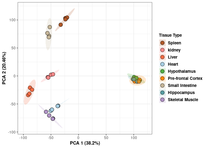
PCA (log Tissue 4wk control)
These plots subset the data so each plot contains mice treated with nothing for 4wks for each tissue.
Scree plot and summary statistics
tdata.FPKM.sample.info <- readRDS(here("Data","20190406_RNAseq_B6_4wk_2DG_counts_phenotypes.RData"))

tdata.FPKM.sample.info.tissue.control.4wk <- rownames_to_column(tdata.FPKM.sample.info) %>% filter(Treatment=="None" & Time=="4 wks") %>% column_to_rownames('rowname')

tdata.FPKM <- readRDS(here("Data","20190406_RNAseq_B6_4wk_2DG_counts_numeric.RData"))

log.tdata.FPKM <- log(tdata.FPKM + 1)
log.tdata.FPKM <- as.data.frame(log.tdata.FPKM)

rows <- rownames(tdata.FPKM.sample.info.tissue.control.4wk)

log.tdata.FPKM.tissue.control.4wk <- rownames_to_column(log.tdata.FPKM)

log.tdata.FPKM.tissue.control.4wk <- log.tdata.FPKM.tissue.control.4wk %>% filter(rowname %in% rows) %>% column_to_rownames('rowname')

pca <- prcomp(log.tdata.FPKM.tissue.control.4wk, center = T)

screeplot(pca,type = "lines")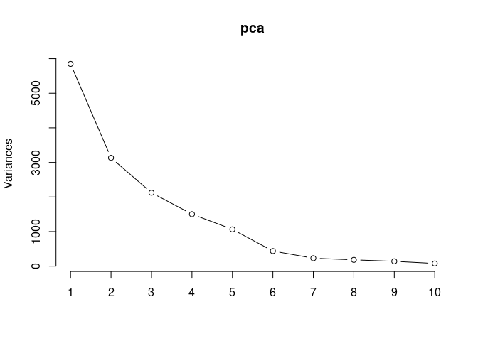
summary(pca)## Importance of components:
## PC1 PC2 PC3 PC4 PC5 PC6
## Standard deviation 76.475 55.9675 46.0808 38.77537 32.6201 20.87983
## Proportion of Variance 0.382 0.2046 0.1387 0.09821 0.0695 0.02848
## Cumulative Proportion 0.382 0.5866 0.7253 0.82353 0.8930 0.92152
## PC7 PC8 PC9 PC10 PC11 PC12
## Standard deviation 15.13501 13.48750 11.82640 8.81376 7.54934 7.45274
## Proportion of Variance 0.01496 0.01188 0.00914 0.00507 0.00372 0.00363
## Cumulative Proportion 0.93648 0.94836 0.95750 0.96257 0.96629 0.96992
## PC13 PC14 PC15 PC16 PC17 PC18 PC19
## Standard deviation 6.6607 6.14877 5.69522 5.61822 5.28325 5.07273 4.89438
## Proportion of Variance 0.0029 0.00247 0.00212 0.00206 0.00182 0.00168 0.00156
## Cumulative Proportion 0.9728 0.97529 0.97741 0.97947 0.98129 0.98297 0.98454
## PC20 PC21 PC22 PC23 PC24 PC25 PC26
## Standard deviation 4.84343 4.70570 4.24727 4.18964 4.03001 3.97337 3.87380
## Proportion of Variance 0.00153 0.00145 0.00118 0.00115 0.00106 0.00103 0.00098
## Cumulative Proportion 0.98607 0.98752 0.98870 0.98984 0.99090 0.99193 0.99292
## PC27 PC28 PC29 PC30 PC31 PC32 PC33
## Standard deviation 3.81601 3.75976 3.68324 3.64879 3.45591 3.37121 3.30757
## Proportion of Variance 0.00095 0.00092 0.00089 0.00087 0.00078 0.00074 0.00071
## Cumulative Proportion 0.99387 0.99479 0.99568 0.99655 0.99733 0.99807 0.99878
## PC34 PC35 PC36
## Standard deviation 3.16594 2.93550 3.396e-14
## Proportion of Variance 0.00065 0.00056 0.000e+00
## Cumulative Proportion 0.99944 1.00000 1.000e+00Tissue
Tissue_color <- as.factor(tdata.FPKM.sample.info.tissue.control.4wk$Tissue)
Tissue_color <- as.data.frame(Tissue_color)
col_tissue <- colorRampPalette(brewer.pal(n = 12, name = "Paired"))(9)[Tissue_color$Tissue_color]
pca_tissue <- cbind(Tissue_color,pca$x[,1],pca$x[,2])
pca_tissue <- as.data.frame(pca_tissue)

p <- ggplot(pca_tissue,aes(pca$x[,1], pca$x[,2]))
p <- p + geom_point(aes(fill = as.factor(pca_tissue$Tissue_color)), shape=21, size=4) + theme_bw()
p <- p + theme(legend.title = element_text(size=10,face="bold")) +
  theme(legend.text = element_text(size=10, face="bold"))
p <- p+ xlab("PCA 1 (38.2%)") + ylab("PCA 2 (20.46%)") + theme(axis.title = element_text(face="bold"))
p <- p + stat_ellipse(aes(pca$x[,1], pca$x[,2], group = Tissue_color, fill = as.factor(pca_tissue$Tissue_color)), geom="polygon",level=0.95,alpha=0.2) +
  scale_fill_manual(values=c("#B15928", "#F88A89", "#F06C45", "#A6CEE3", "#52AF43", "#FE870D", "#C7B699", "#569EA4","#B294C7"),name="Tissue Type",
                       breaks=c("Spleen", "Kidney","Liver","Heart","Hypothanamus","Pre-frontal Cortex","Small Intestine","Hippocampus","Skeletal Muscle"),
                       labels=c("Spleen", "kidney","Liver","Heart","Hypothalamus","Pre-frontal Cortex","Small Intestine","Hippocampus","Skeletal Muscle")) +
  scale_linetype_manual(values=c(1,2,1,2,1))
print(p)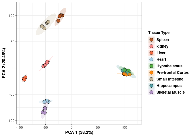
PCA (log Treatment by tissue 96hr)
These plots subset the data so each plot contains mice that were treated or untreated for 96hrs for each tissue.
Scree plot and summary statistics Spleen
tdata.FPKM.sample.info <- readRDS(here("Data","20190406_RNAseq_B6_4wk_2DG_counts_phenotypes.RData"))

tdata.FPKM.sample.info.spleen <- rownames_to_column(tdata.FPKM.sample.info) %>% filter(Tissue=="Spleen" & Time=="96 hrs") %>% column_to_rownames('rowname')

tdata.FPKM <- readRDS(here("Data","20190406_RNAseq_B6_4wk_2DG_counts_numeric.RData"))

log.tdata.FPKM <- log(tdata.FPKM + 1)
log.tdata.FPKM <- as.data.frame(log.tdata.FPKM)

rows <- rownames(tdata.FPKM.sample.info.spleen)

log.tdata.FPKM.spleen <- rownames_to_column(log.tdata.FPKM)

log.tdata.FPKM.spleen <- log.tdata.FPKM.spleen %>% filter(rowname %in% rows) %>% column_to_rownames('rowname')

pca <- prcomp(log.tdata.FPKM.spleen, center = T)

screeplot(pca,type = "lines")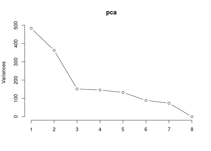
summary(pca)## Importance of components:
## PC1 PC2 PC3 PC4 PC5 PC6 PC7
## Standard deviation 21.976 19.0388 12.3062 12.0731 11.49332 9.43497 8.57260
## Proportion of Variance 0.336 0.2522 0.1054 0.1014 0.09191 0.06194 0.05113
## Cumulative Proportion 0.336 0.5882 0.6936 0.7950 0.88693 0.94887 1.00000
## PC8
## Standard deviation 1.768e-14
## Proportion of Variance 0.000e+00
## Cumulative Proportion 1.000e+00Treatment Spleen
Treatment_color <- as.factor(tdata.FPKM.sample.info.spleen$Treatment)
Treatment_color <- as.data.frame(Treatment_color)
col_treatment <- colorRampPalette(brewer.pal(n = 12, name = "Paired"))(2)[Treatment_color$Treatment_color]
pca_treatment <- cbind(Treatment_color,pca$x[,1],pca$x[,2])
pca_treatment <- as.data.frame(pca_treatment)

p <- ggplot(pca_treatment,aes(pca$x[,1], pca$x[,2]))
p <- p + geom_point(aes(fill = as.factor(pca_treatment$Treatment_color)), shape=21, size=4) + theme_bw()
p <- p + theme(legend.title = element_text(size=10,face="bold")) +
  theme(legend.text = element_text(size=10, face="bold"))
p <- p + xlab("PCA 1 (33.6%)") + ylab("PCA 2 (25.22%)") + theme(axis.title = element_text(face="bold"))
p <- p + stat_ellipse(aes(pca$x[,1], pca$x[,2], group = Treatment_color, fill = as.factor(pca_treatment$Treatment_color)), geom="polygon",level=0.95,alpha=0.4) +
  scale_fill_manual(values=c("#A6CEE3", "#B15928"),name="Treatment Type",
                       breaks=c("2DG", "None"),
                       labels=c("2DG", "Control")) +
  scale_linetype_manual(values=c(1,2))
print(p)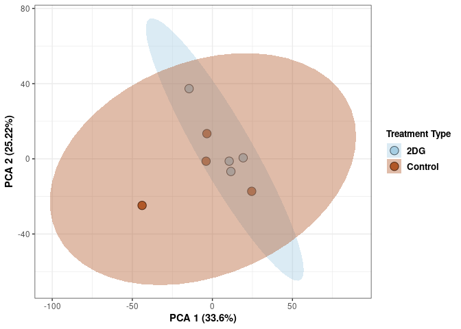
Scree plot and summary statistics kidney
tdata.FPKM.sample.info <- readRDS(here("Data","20190406_RNAseq_B6_4wk_2DG_counts_phenotypes.RData"))

tdata.FPKM.sample.info.kidney <- rownames_to_column(tdata.FPKM.sample.info) %>% filter(Tissue=="Kidney" & Time=="96 hrs") %>% column_to_rownames('rowname')

tdata.FPKM <- readRDS(here("Data","20190406_RNAseq_B6_4wk_2DG_counts_numeric.RData"))

log.tdata.FPKM <- log(tdata.FPKM + 1)
log.tdata.FPKM <- as.data.frame(log.tdata.FPKM)

rows <- rownames(tdata.FPKM.sample.info.kidney)

log.tdata.FPKM.kidney <- rownames_to_column(log.tdata.FPKM)

log.tdata.FPKM.kidney <- log.tdata.FPKM.kidney %>% filter(rowname %in% rows) %>% column_to_rownames('rowname')

pca <- prcomp(log.tdata.FPKM.kidney, center = T)

screeplot(pca,type = "lines")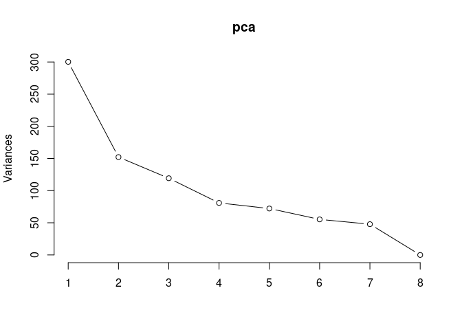
summary(pca)## Importance of components:
## PC1 PC2 PC3 PC4 PC5 PC6 PC7
## Standard deviation 17.3265 12.3355 10.9207 8.99281 8.4963 7.43458 6.91577
## Proportion of Variance 0.3627 0.1838 0.1441 0.09769 0.0872 0.06677 0.05778
## Cumulative Proportion 0.3627 0.5465 0.6905 0.78825 0.8754 0.94222 1.00000
## PC8
## Standard deviation 1.565e-14
## Proportion of Variance 0.000e+00
## Cumulative Proportion 1.000e+00Treatment kidney
Treatment_color <- as.factor(tdata.FPKM.sample.info.kidney$Treatment)
Treatment_color <- as.data.frame(Treatment_color)
col_treatment <- colorRampPalette(brewer.pal(n = 12, name = "Paired"))(2)[Treatment_color$Treatment_color]
pca_treatment <- cbind(Treatment_color,pca$x[,1],pca$x[,2])
pca_treatment <- as.data.frame(pca_treatment)

p <- ggplot(pca_treatment,aes(pca$x[,1], pca$x[,2]))
p <- p + geom_point(aes(fill = as.factor(pca_treatment$Treatment_color)), shape=21, size=4) + theme_bw()
p <- p + theme(legend.title = element_text(size=10,face="bold")) +
  theme(legend.text = element_text(size=10, face="bold"))
p <- p + xlab("PCA 1 (36.27%)") + ylab("PCA 2 (18.38%)") + theme(axis.title = element_text(face="bold"))
p <- p + stat_ellipse(aes(pca$x[,1], pca$x[,2], group = Treatment_color, fill = as.factor(pca_treatment$Treatment_color)), geom="polygon",level=0.95,alpha=0.4) +
  scale_fill_manual(values=c("#A6CEE3", "#B15928"),name="Treatment Type",
                       breaks=c("2DG", "None"),
                       labels=c("2DG", "Control")) +
  scale_linetype_manual(values=c(1,2))
print(p)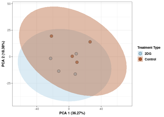
Scree plot and summary statistics hypothalamus
tdata.FPKM.sample.info <- readRDS(here("Data","20190406_RNAseq_B6_4wk_2DG_counts_phenotypes.RData"))

tdata.FPKM.sample.info.hypothalamus <- rownames_to_column(tdata.FPKM.sample.info) %>% filter(Tissue=="Hypothanamus" & Time=="96 hrs") %>% column_to_rownames('rowname')

tdata.FPKM <- readRDS(here("Data","20190406_RNAseq_B6_4wk_2DG_counts_numeric.RData"))

log.tdata.FPKM <- log(tdata.FPKM + 1)
log.tdata.FPKM <- as.data.frame(log.tdata.FPKM)

rows <- rownames(tdata.FPKM.sample.info.hypothalamus)

log.tdata.FPKM.hypothalamus <- rownames_to_column(log.tdata.FPKM)

log.tdata.FPKM.hypothalamus <- log.tdata.FPKM.hypothalamus %>% filter(rowname %in% rows) %>% column_to_rownames('rowname')

pca <- prcomp(log.tdata.FPKM.hypothalamus, center = T)

screeplot(pca,type = "lines")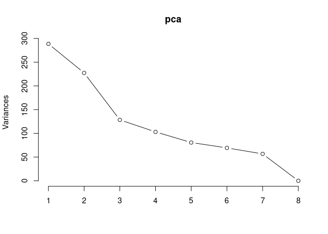
summary(pca)## Importance of components:
## PC1 PC2 PC3 PC4 PC5 PC6 PC7
## Standard deviation 16.9867 15.0757 11.3299 10.1493 8.9774 8.32471 7.52753
## Proportion of Variance 0.3025 0.2383 0.1346 0.1080 0.0845 0.07266 0.05941
## Cumulative Proportion 0.3025 0.5408 0.6754 0.7834 0.8679 0.94059 1.00000
## PC8
## Standard deviation 1.739e-14
## Proportion of Variance 0.000e+00
## Cumulative Proportion 1.000e+00Treatment hypothalamus
Treatment_color <- as.factor(tdata.FPKM.sample.info.hypothalamus$Treatment)
Treatment_color <- as.data.frame(Treatment_color)
col_treatment <- colorRampPalette(brewer.pal(n = 12, name = "Paired"))(2)[Treatment_color$Treatment_color]
pca_treatment <- cbind(Treatment_color,pca$x[,1],pca$x[,2])
pca_treatment <- as.data.frame(pca_treatment)

p <- ggplot(pca_treatment,aes(pca$x[,1], pca$x[,2]))
p <- p + geom_point(aes(fill = as.factor(pca_treatment$Treatment_color)), shape=21, size=4) + theme_bw()
p <- p + theme(legend.title = element_text(size=10,face="bold")) +
  theme(legend.text = element_text(size=10, face="bold"))
p <- p + xlab("PCA 1 (30.25%)") + ylab("PCA 2 (23.83%)") + theme(axis.title = element_text(face="bold"))
p <- p + stat_ellipse(aes(pca$x[,1], pca$x[,2], group = Treatment_color, fill = as.factor(pca_treatment$Treatment_color)), geom="polygon",level=0.95,alpha=0.4) +
  scale_fill_manual(values=c("#A6CEE3", "#B15928"),name="Treatment Type",
                       breaks=c("2DG", "None"),
                       labels=c("2DG", "Control")) +
  scale_linetype_manual(values=c(1,2))
print(p)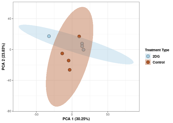
Scree plot and summary statistics hippocampus
tdata.FPKM.sample.info <- readRDS(here("Data","20190406_RNAseq_B6_4wk_2DG_counts_phenotypes.RData"))

tdata.FPKM.sample.info.hippocampus <- rownames_to_column(tdata.FPKM.sample.info) %>% filter(Tissue=="Hippocampus" & Time=="96 hrs") %>% column_to_rownames('rowname')

tdata.FPKM <- readRDS(here("Data","20190406_RNAseq_B6_4wk_2DG_counts_numeric.RData"))

log.tdata.FPKM <- log(tdata.FPKM + 1)
log.tdata.FPKM <- as.data.frame(log.tdata.FPKM)

rows <- rownames(tdata.FPKM.sample.info.hippocampus)

log.tdata.FPKM.hippocampus <- rownames_to_column(log.tdata.FPKM)

log.tdata.FPKM.hippocampus <- log.tdata.FPKM.hippocampus %>% filter(rowname %in% rows) %>% column_to_rownames('rowname')

pca <- prcomp(log.tdata.FPKM.hippocampus, center = T)

screeplot(pca,type = "lines")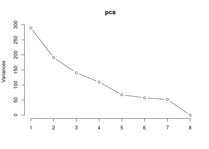
summary(pca)## Importance of components:
## PC1 PC2 PC3 PC4 PC5 PC6 PC7
## Standard deviation 17.013 13.8240 11.8542 10.4775 8.21732 7.57485 7.19112
## Proportion of Variance 0.319 0.2106 0.1548 0.1210 0.07441 0.06323 0.05699
## Cumulative Proportion 0.319 0.5295 0.6844 0.8054 0.87979 0.94301 1.00000
## PC8
## Standard deviation 1.73e-14
## Proportion of Variance 0.00e+00
## Cumulative Proportion 1.00e+00Treatment hippocampus
Treatment_color <- as.factor(tdata.FPKM.sample.info.hippocampus$Treatment)
Treatment_color <- as.data.frame(Treatment_color)
col_treatment <- colorRampPalette(brewer.pal(n = 12, name = "Paired"))(2)[Treatment_color$Treatment_color]
pca_treatment <- cbind(Treatment_color,pca$x[,1],pca$x[,2])
pca_treatment <- as.data.frame(pca_treatment)

p <- ggplot(pca_treatment,aes(pca$x[,1], pca$x[,2]))
p <- p + geom_point(aes(fill = as.factor(pca_treatment$Treatment_color)), shape=21, size=4) + theme_bw()
p <- p + theme(legend.title = element_text(size=10,face="bold")) +
  theme(legend.text = element_text(size=10, face="bold"))
p <- p + xlab("PCA 1 (31.9%)") + ylab("PCA 2 (21.06%)") + theme(axis.title = element_text(face="bold"))
p <- p + stat_ellipse(aes(pca$x[,1], pca$x[,2], group = Treatment_color, fill = as.factor(pca_treatment$Treatment_color)), geom="polygon",level=0.95,alpha=0.4) +
  scale_fill_manual(values=c("#A6CEE3", "#B15928"),name="Treatment Type",
                       breaks=c("2DG", "None"),
                       labels=c("2DG", "Control")) +
  scale_linetype_manual(values=c(1,2))
print(p)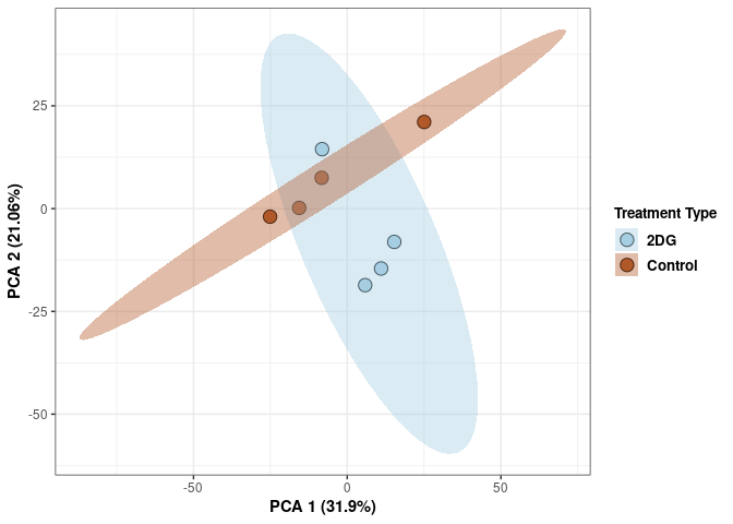
Scree plot and summary statistics liver
tdata.FPKM.sample.info <- readRDS(here("Data","20190406_RNAseq_B6_4wk_2DG_counts_phenotypes.RData"))

tdata.FPKM.sample.info.liver <- rownames_to_column(tdata.FPKM.sample.info) %>% filter(Tissue=="Liver" & Time=="96 hrs") %>% column_to_rownames('rowname')

tdata.FPKM <- readRDS(here("Data","20190406_RNAseq_B6_4wk_2DG_counts_numeric.RData"))

log.tdata.FPKM <- log(tdata.FPKM + 1)
log.tdata.FPKM <- as.data.frame(log.tdata.FPKM)

rows <- rownames(tdata.FPKM.sample.info.liver)

log.tdata.FPKM.liver <- rownames_to_column(log.tdata.FPKM)

log.tdata.FPKM.liver <- log.tdata.FPKM.liver %>% filter(rowname %in% rows) %>% column_to_rownames('rowname')

pca <- prcomp(log.tdata.FPKM.liver, center = T)

screeplot(pca,type = "lines")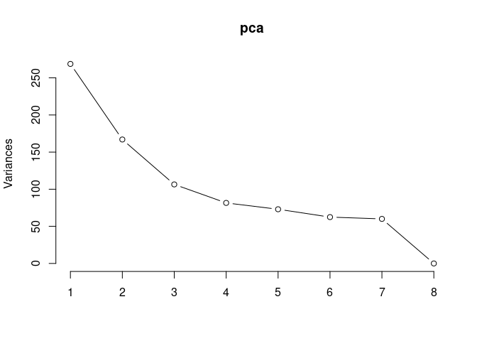
summary(pca)## Importance of components:
## PC1 PC2 PC3 PC4 PC5 PC6 PC7
## Standard deviation 16.3947 12.9218 10.3181 9.02994 8.54420 7.90209 7.74698
## Proportion of Variance 0.3281 0.2038 0.1300 0.09953 0.08911 0.07622 0.07326
## Cumulative Proportion 0.3281 0.5319 0.6619 0.76141 0.85052 0.92674 1.00000
## PC8
## Standard deviation 1.4e-14
## Proportion of Variance 0.0e+00
## Cumulative Proportion 1.0e+00Treatment liver
Treatment_color <- as.factor(tdata.FPKM.sample.info.liver$Treatment)
Treatment_color <- as.data.frame(Treatment_color)
col_treatment <- colorRampPalette(brewer.pal(n = 12, name = "Paired"))(2)[Treatment_color$Treatment_color]
pca_treatment <- cbind(Treatment_color,pca$x[,1],pca$x[,2])
pca_treatment <- as.data.frame(pca_treatment)

p <- ggplot(pca_treatment,aes(pca$x[,1], pca$x[,2]))
p <- p + geom_point(aes(fill = as.factor(pca_treatment$Treatment_color)), shape=21, size=4) + theme_bw()
p <- p + theme(legend.title = element_text(size=10,face="bold")) +
  theme(legend.text = element_text(size=10, face="bold"))
p <- p + xlab("PCA 1 (32.81%)") + ylab("PCA 2 (20.38%)") + theme(axis.title = element_text(face="bold"))
p <- p + stat_ellipse(aes(pca$x[,1], pca$x[,2], group = Treatment_color, fill = as.factor(pca_treatment$Treatment_color)), geom="polygon",level=0.95,alpha=0.4) +
  scale_fill_manual(values=c("#A6CEE3", "#B15928"),name="Treatment Type",
                       breaks=c("2DG", "None"),
                       labels=c("2DG", "Control")) +
  scale_linetype_manual(values=c(1,2))
print(p)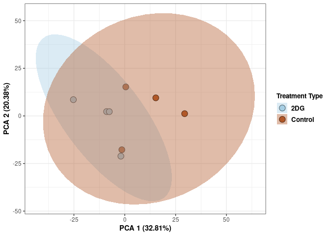
Scree plot and summary statistics heart
tdata.FPKM.sample.info <- readRDS(here("Data","20190406_RNAseq_B6_4wk_2DG_counts_phenotypes.RData"))

tdata.FPKM.sample.info.heart <- rownames_to_column(tdata.FPKM.sample.info) %>% filter(Tissue=="Heart" & Time=="96 hrs") %>% column_to_rownames('rowname')

tdata.FPKM <- readRDS(here("Data","20190406_RNAseq_B6_4wk_2DG_counts_numeric.RData"))

log.tdata.FPKM <- log(tdata.FPKM + 1)
log.tdata.FPKM <- as.data.frame(log.tdata.FPKM)

rows <- rownames(tdata.FPKM.sample.info.heart)

log.tdata.FPKM.heart <- rownames_to_column(log.tdata.FPKM)

log.tdata.FPKM.heart <- log.tdata.FPKM.heart %>% filter(rowname %in% rows) %>% column_to_rownames('rowname')

pca <- prcomp(log.tdata.FPKM.heart, center = T)

screeplot(pca,type = "lines")
summary(pca)## Importance of components:
## PC1 PC2 PC3 PC4 PC5 PC6 PC7
## Standard deviation 19.0795 14.0520 12.7659 8.70533 7.92699 7.49191 7.42554
## Proportion of Variance 0.3736 0.2027 0.1673 0.07778 0.06449 0.05761 0.05659
## Cumulative Proportion 0.3736 0.5763 0.7435 0.82131 0.88580 0.94341 1.00000
## PC8
## Standard deviation 1.326e-14
## Proportion of Variance 0.000e+00
## Cumulative Proportion 1.000e+00Treatment heart
Treatment_color <- as.factor(tdata.FPKM.sample.info.heart$Treatment)
Treatment_color <- as.data.frame(Treatment_color)
col_treatment <- colorRampPalette(brewer.pal(n = 12, name = "Paired"))(2)[Treatment_color$Treatment_color]
pca_treatment <- cbind(Treatment_color,pca$x[,1],pca$x[,2])
pca_treatment <- as.data.frame(pca_treatment)

p <- ggplot(pca_treatment,aes(pca$x[,1], pca$x[,2]))
p <- p + geom_point(aes(fill = as.factor(pca_treatment$Treatment_color)), shape=21, size=4) + theme_bw()
p <- p + theme(legend.title = element_text(size=10,face="bold")) +
  theme(legend.text = element_text(size=10, face="bold"))
p <- p + xlab("PCA 1 (37.36%)") + ylab("PCA 2 (20.27%)") + theme(axis.title = element_text(face="bold"))
p <- p + stat_ellipse(aes(pca$x[,1], pca$x[,2], group = Treatment_color, fill = as.factor(pca_treatment$Treatment_color)), geom="polygon",level=0.95,alpha=0.4) +
  scale_fill_manual(values=c("#A6CEE3", "#B15928"),name="Treatment Type",
                       breaks=c("2DG", "None"),
                       labels=c("2DG", "Control")) +
  scale_linetype_manual(values=c(1,2))
print(p)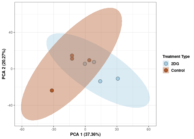
Scree plot and summary statistics small intestine
tdata.FPKM.sample.info <- readRDS(here("Data","20190406_RNAseq_B6_4wk_2DG_counts_phenotypes.RData"))

tdata.FPKM.sample.info.small.intestine <- rownames_to_column(tdata.FPKM.sample.info) %>% filter(Tissue=="Small Intestine" & Time=="96 hrs") %>% column_to_rownames('rowname')

tdata.FPKM <- readRDS(here("Data","20190406_RNAseq_B6_4wk_2DG_counts_numeric.RData"))

log.tdata.FPKM <- log(tdata.FPKM + 1)
log.tdata.FPKM <- as.data.frame(log.tdata.FPKM)

rows <- rownames(tdata.FPKM.sample.info.small.intestine)

log.tdata.FPKM.small.intestine <- rownames_to_column(log.tdata.FPKM)

log.tdata.FPKM.small.intestine <- log.tdata.FPKM.small.intestine %>% filter(rowname %in% rows) %>% column_to_rownames('rowname')

pca <- prcomp(log.tdata.FPKM.small.intestine, center = T)

screeplot(pca,type = "lines")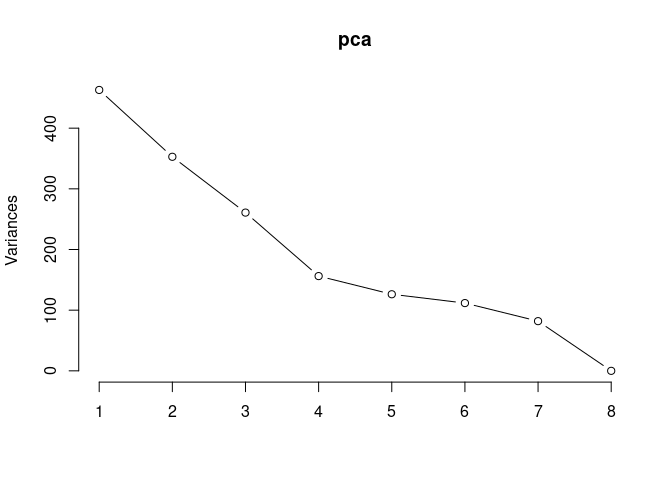
summary(pca)## Importance of components:
## PC1 PC2 PC3 PC4 PC5 PC6 PC7
## Standard deviation 21.5167 18.7833 16.1506 12.4971 11.2351 10.56847 9.05043
## Proportion of Variance 0.2982 0.2272 0.1680 0.1006 0.0813 0.07194 0.05276
## Cumulative Proportion 0.2982 0.5254 0.6934 0.7940 0.8753 0.94724 1.00000
## PC8
## Standard deviation 1.708e-14
## Proportion of Variance 0.000e+00
## Cumulative Proportion 1.000e+00Treatment small intestine
Treatment_color <- as.factor(tdata.FPKM.sample.info.small.intestine$Treatment)
Treatment_color <- as.data.frame(Treatment_color)
col_treatment <- colorRampPalette(brewer.pal(n = 12, name = "Paired"))(2)[Treatment_color$Treatment_color]
pca_treatment <- cbind(Treatment_color,pca$x[,1],pca$x[,2])
pca_treatment <- as.data.frame(pca_treatment)

p <- ggplot(pca_treatment,aes(pca$x[,1], pca$x[,2]))
p <- p + geom_point(aes(fill = as.factor(pca_treatment$Treatment_color)), shape=21, size=4) + theme_bw()
p <- p + theme(legend.title = element_text(size=10,face="bold")) +
  theme(legend.text = element_text(size=10, face="bold"))
p <- p + xlab("PCA 1 (29.82%)") + ylab("PCA 2 (22.72%)") + theme(axis.title = element_text(face="bold"))
p <- p + stat_ellipse(aes(pca$x[,1], pca$x[,2], group = Treatment_color, fill = as.factor(pca_treatment$Treatment_color)), geom="polygon",level=0.95,alpha=0.4) +
  scale_fill_manual(values=c("#A6CEE3", "#B15928"),name="Treatment Type",
                       breaks=c("2DG", "None"),
                       labels=c("2DG", "Control")) +
  scale_linetype_manual(values=c(1,2))
print(p)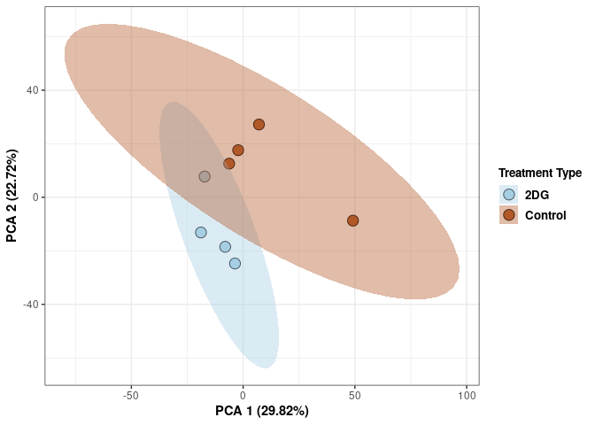
Scree plot and summary statistics skeletal muscle
tdata.FPKM.sample.info <- readRDS(here("Data","20190406_RNAseq_B6_4wk_2DG_counts_phenotypes.RData"))

tdata.FPKM.sample.info.skeletal.muscle <- rownames_to_column(tdata.FPKM.sample.info) %>% filter(Tissue=="Skeletal Muscle" & Time=="96 hrs") %>% column_to_rownames('rowname')

tdata.FPKM <- readRDS(here("Data","20190406_RNAseq_B6_4wk_2DG_counts_numeric.RData"))

log.tdata.FPKM <- log(tdata.FPKM + 1)
log.tdata.FPKM <- as.data.frame(log.tdata.FPKM)

rows <- rownames(tdata.FPKM.sample.info.skeletal.muscle)

log.tdata.FPKM.skeletal.muscle <- rownames_to_column(log.tdata.FPKM)

log.tdata.FPKM.skeletal.muscle <- log.tdata.FPKM.skeletal.muscle %>% filter(rowname %in% rows) %>% column_to_rownames('rowname')

pca <- prcomp(log.tdata.FPKM.skeletal.muscle, center = T)

screeplot(pca,type = "lines")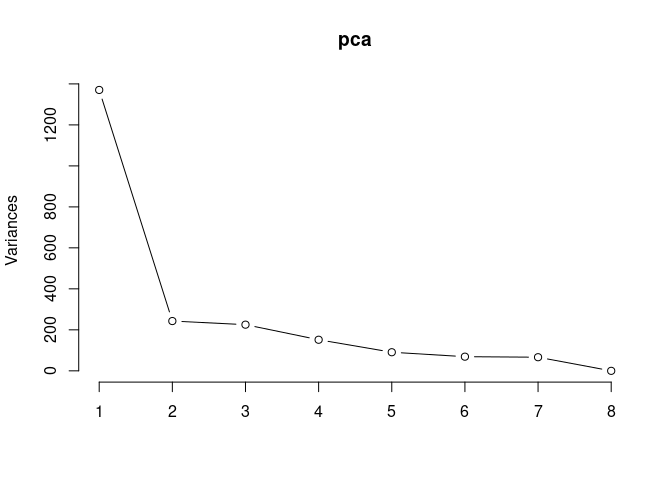
summary(pca)## Importance of components:
## PC1 PC2 PC3 PC4 PC5 PC6 PC7
## Standard deviation 37.0186 15.5860 15.0101 12.31690 9.52859 8.31463 8.155
## Proportion of Variance 0.6182 0.1096 0.1016 0.06844 0.04096 0.03119 0.030
## Cumulative Proportion 0.6182 0.7278 0.8294 0.89786 0.93882 0.97000 1.000
## PC8
## Standard deviation 1.453e-14
## Proportion of Variance 0.000e+00
## Cumulative Proportion 1.000e+00Treatment skeletal muscle
Treatment_color <- as.factor(tdata.FPKM.sample.info.skeletal.muscle$Treatment)
Treatment_color <- as.data.frame(Treatment_color)
col_treatment <- colorRampPalette(brewer.pal(n = 12, name = "Paired"))(2)[Treatment_color$Treatment_color]
pca_treatment <- cbind(Treatment_color,pca$x[,1],pca$x[,2])
pca_treatment <- as.data.frame(pca_treatment)

p <- ggplot(pca_treatment,aes(pca$x[,1], pca$x[,2]))
p <- p + geom_point(aes(fill = as.factor(pca_treatment$Treatment_color)), shape=21, size=4) + theme_bw()
p <- p + theme(legend.title = element_text(size=10,face="bold")) +
  theme(legend.text = element_text(size=10, face="bold"))
p <- p + xlab("PCA 1 (61.82%)") + ylab("PCA 2 (10.96%)") + theme(axis.title = element_text(face="bold"))
p <- p + stat_ellipse(aes(pca$x[,1], pca$x[,2], group = Treatment_color, fill = as.factor(pca_treatment$Treatment_color)), geom="polygon",level=0.95,alpha=0.4) +
  scale_fill_manual(values=c("#A6CEE3", "#B15928"),name="Treatment Type",
                       breaks=c("2DG", "None"),
                       labels=c("2DG", "Control")) +
  scale_linetype_manual(values=c(1,2))
print(p)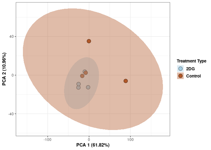
Scree plot and summary statistics prefrontal cortex
tdata.FPKM.sample.info <- readRDS(here("Data","20190406_RNAseq_B6_4wk_2DG_counts_phenotypes.RData"))

tdata.FPKM.sample.info.prefrontal.cortex <- rownames_to_column(tdata.FPKM.sample.info) %>% filter(Tissue=="Pre-frontal Cortex" & Time=="96 hrs") %>% column_to_rownames('rowname')

tdata.FPKM <- readRDS(here("Data","20190406_RNAseq_B6_4wk_2DG_counts_numeric.RData"))

log.tdata.FPKM <- log(tdata.FPKM + 1)
log.tdata.FPKM <- as.data.frame(log.tdata.FPKM)

rows <- rownames(tdata.FPKM.sample.info.prefrontal.cortex)

log.tdata.FPKM.prefrontal.cortex <- rownames_to_column(log.tdata.FPKM)

log.tdata.FPKM.prefrontal.cortex <- log.tdata.FPKM.prefrontal.cortex %>% filter(rowname %in% rows) %>% column_to_rownames('rowname')

pca <- prcomp(log.tdata.FPKM.prefrontal.cortex, center = T)

screeplot(pca,type = "lines")
summary(pca)## Importance of components:
## PC1 PC2 PC3 PC4 PC5 PC6 PC7
## Standard deviation 20.976 17.0942 12.3296 10.14394 8.65608 8.11665 7.39452
## Proportion of Variance 0.372 0.2471 0.1285 0.08701 0.06336 0.05571 0.04624
## Cumulative Proportion 0.372 0.6191 0.7477 0.83470 0.89806 0.95376 1.00000
## PC8
## Standard deviation 1.748e-14
## Proportion of Variance 0.000e+00
## Cumulative Proportion 1.000e+00Treatment prefrontal cortex
Treatment_color <- as.factor(tdata.FPKM.sample.info.prefrontal.cortex$Treatment)
Treatment_color <- as.data.frame(Treatment_color)
col_treatment <- colorRampPalette(brewer.pal(n = 12, name = "Paired"))(2)[Treatment_color$Treatment_color]
pca_treatment <- cbind(Treatment_color,pca$x[,1],pca$x[,2])
pca_treatment <- as.data.frame(pca_treatment)

p <- ggplot(pca_treatment,aes(pca$x[,1], pca$x[,2]))
p <- p + geom_point(aes(fill = as.factor(pca_treatment$Treatment_color)), shape=21, size=4) + theme_bw()
p <- p + theme(legend.title = element_text(size=10,face="bold")) +
  theme(legend.text = element_text(size=10, face="bold"))
p <- p + xlab("PCA 1 (37.2%)") + ylab("PCA 2 (24.71%)") + theme(axis.title = element_text(face="bold"))
p <- p + stat_ellipse(aes(pca$x[,1], pca$x[,2], group = Treatment_color, fill = as.factor(pca_treatment$Treatment_color)), geom="polygon",level=0.95,alpha=0.4) +
  scale_fill_manual(values=c("#A6CEE3", "#B15928"),name="Treatment Type",
                       breaks=c("2DG", "None"),
                       labels=c("2DG", "Control")) +
  scale_linetype_manual(values=c(1,2))
print(p)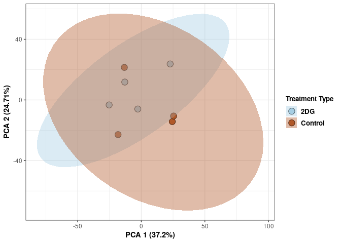
PCA (log Treatment by tissue 4wk)
These plots subset the data so each plot contains mice that were treated or untreated for 4wks for each tissue.
Scree plot and summary statistics Spleen
tdata.FPKM.sample.info <- readRDS(here("Data","20190406_RNAseq_B6_4wk_2DG_counts_phenotypes.RData"))

tdata.FPKM.sample.info.spleen <- rownames_to_column(tdata.FPKM.sample.info) %>% filter(Tissue=="Spleen" & Time=="4 wks") %>% column_to_rownames('rowname')

tdata.FPKM <- readRDS(here("Data","20190406_RNAseq_B6_4wk_2DG_counts_numeric.RData"))

log.tdata.FPKM <- log(tdata.FPKM + 1)
log.tdata.FPKM <- as.data.frame(log.tdata.FPKM)

rows <- rownames(tdata.FPKM.sample.info.spleen)

log.tdata.FPKM.spleen <- rownames_to_column(log.tdata.FPKM)

log.tdata.FPKM.spleen <- log.tdata.FPKM.spleen %>% filter(rowname %in% rows) %>% column_to_rownames('rowname')

pca <- prcomp(log.tdata.FPKM.spleen, center = T)

screeplot(pca,type = "lines")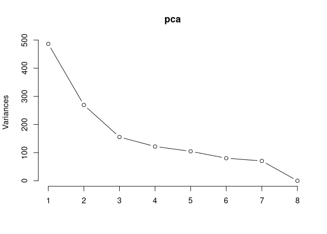
summary(pca)## Importance of components:
## PC1 PC2 PC3 PC4 PC5 PC6
## Standard deviation 22.0563 16.4096 12.4704 11.03395 10.23196 8.95618
## Proportion of Variance 0.3776 0.2090 0.1207 0.09449 0.08126 0.06226
## Cumulative Proportion 0.3776 0.5866 0.7073 0.80175 0.88300 0.94526
## PC7 PC8
## Standard deviation 8.39820 1.79e-14
## Proportion of Variance 0.05474 0.00e+00
## Cumulative Proportion 1.00000 1.00e+00Treatment Spleen
Treatment_color <- as.factor(tdata.FPKM.sample.info.spleen$Treatment)
Treatment_color <- as.data.frame(Treatment_color)
col_treatment <- colorRampPalette(brewer.pal(n = 12, name = "Paired"))(2)[Treatment_color$Treatment_color]
pca_treatment <- cbind(Treatment_color,pca$x[,1],pca$x[,2])
pca_treatment <- as.data.frame(pca_treatment)

p <- ggplot(pca_treatment,aes(pca$x[,1], pca$x[,2]))
p <- p + geom_point(aes(fill = as.factor(pca_treatment$Treatment_color)), shape=21, size=4) + theme_bw()
p <- p + theme(legend.title = element_text(size=10,face="bold")) +
  theme(legend.text = element_text(size=10, face="bold"))
p <- p + xlab("PCA 1 (37.76%)") + ylab("PCA 2 (20.90%)") + theme(axis.title = element_text(face="bold"))
p <- p + stat_ellipse(aes(pca$x[,1], pca$x[,2], group = Treatment_color, fill = as.factor(pca_treatment$Treatment_color)), geom="polygon",level=0.95,alpha=0.4) +
  scale_fill_manual(values=c("#A6CEE3", "#B15928"),name="Treatment Type",
                       breaks=c("2DG", "None"),
                       labels=c("2DG", "Control")) +
  scale_linetype_manual(values=c(1,2))
print(p)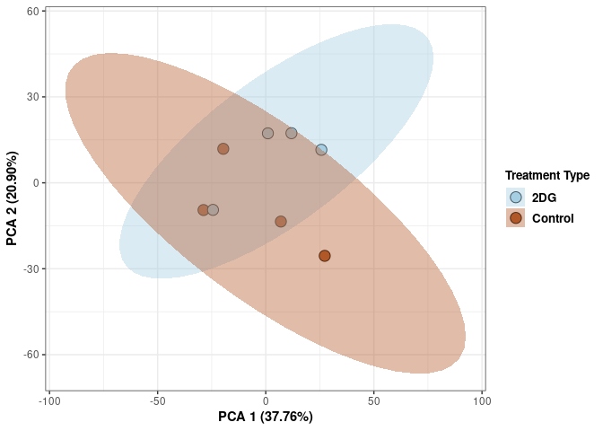
Scree plot and summary statistics kidney
tdata.FPKM.sample.info <- readRDS(here("Data","20190406_RNAseq_B6_4wk_2DG_counts_phenotypes.RData"))

tdata.FPKM.sample.info.kidney <- rownames_to_column(tdata.FPKM.sample.info) %>% filter(Tissue=="Kidney" & Time=="4 wks") %>% column_to_rownames('rowname')

tdata.FPKM <- readRDS(here("Data","20190406_RNAseq_B6_4wk_2DG_counts_numeric.RData"))

log.tdata.FPKM <- log(tdata.FPKM + 1)
log.tdata.FPKM <- as.data.frame(log.tdata.FPKM)

rows <- rownames(tdata.FPKM.sample.info.kidney)

log.tdata.FPKM.kidney <- rownames_to_column(log.tdata.FPKM)

log.tdata.FPKM.kidney <- log.tdata.FPKM.kidney %>% filter(rowname %in% rows) %>% column_to_rownames('rowname')

pca <- prcomp(log.tdata.FPKM.kidney, center = T)

screeplot(pca,type = "lines")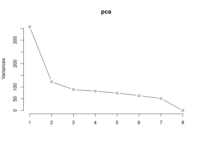
summary(pca)## Importance of components:
## PC1 PC2 PC3 PC4 PC5 PC6 PC7
## Standard deviation 18.8991 11.0609 9.4461 9.08241 8.61244 7.97630 7.12982
## Proportion of Variance 0.4253 0.1457 0.1062 0.09822 0.08832 0.07575 0.06053
## Cumulative Proportion 0.4253 0.5709 0.6772 0.77541 0.86372 0.93947 1.00000
## PC8
## Standard deviation 1.571e-14
## Proportion of Variance 0.000e+00
## Cumulative Proportion 1.000e+00Treatment kidney
Treatment_color <- as.factor(tdata.FPKM.sample.info.kidney$Treatment)
Treatment_color <- as.data.frame(Treatment_color)
col_treatment <- colorRampPalette(brewer.pal(n = 12, name = "Paired"))(2)[Treatment_color$Treatment_color]
pca_treatment <- cbind(Treatment_color,pca$x[,1],pca$x[,2])
pca_treatment <- as.data.frame(pca_treatment)

p <- ggplot(pca_treatment,aes(pca$x[,1], pca$x[,2]))
p <- p + geom_point(aes(fill = as.factor(pca_treatment$Treatment_color)), shape=21, size=4) + theme_bw()
p <- p + theme(legend.title = element_text(size=10,face="bold")) +
  theme(legend.text = element_text(size=10, face="bold"))
p <- p + xlab("PCA 1 (42.53%)") + ylab("PCA 2 (14.57%)") + theme(axis.title = element_text(face="bold"))
p <- p + stat_ellipse(aes(pca$x[,1], pca$x[,2], group = Treatment_color, fill = as.factor(pca_treatment$Treatment_color)), geom="polygon",level=0.95,alpha=0.4) +
  scale_fill_manual(values=c("#A6CEE3", "#B15928"),name="Treatment Type",
                       breaks=c("2DG", "None"),
                       labels=c("2DG", "Control")) +
  scale_linetype_manual(values=c(1,2))
print(p)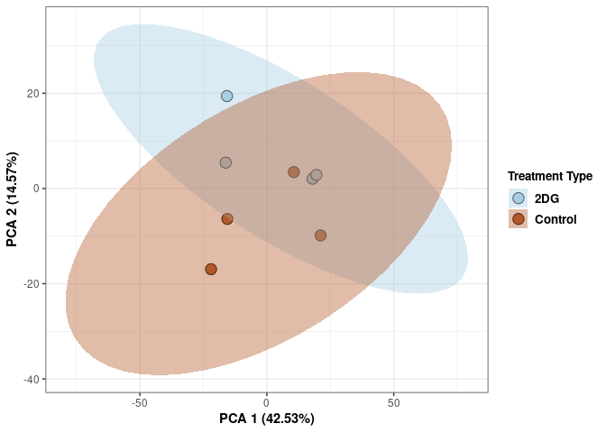
Scree plot and summary statistics hypothalamus
tdata.FPKM.sample.info <- readRDS(here("Data","20190406_RNAseq_B6_4wk_2DG_counts_phenotypes.RData"))

tdata.FPKM.sample.info.hypothalamus <- rownames_to_column(tdata.FPKM.sample.info) %>% filter(Tissue=="Hypothanamus" & Time=="4 wks") %>% column_to_rownames('rowname')

tdata.FPKM <- readRDS(here("Data","20190406_RNAseq_B6_4wk_2DG_counts_numeric.RData"))

log.tdata.FPKM <- log(tdata.FPKM + 1)
log.tdata.FPKM <- as.data.frame(log.tdata.FPKM)

rows <- rownames(tdata.FPKM.sample.info.hypothalamus)

log.tdata.FPKM.hypothalamus <- rownames_to_column(log.tdata.FPKM)

log.tdata.FPKM.hypothalamus <- log.tdata.FPKM.hypothalamus %>% filter(rowname %in% rows) %>% column_to_rownames('rowname')

pca <- prcomp(log.tdata.FPKM.hypothalamus, center = T)

screeplot(pca,type = "lines")
summary(pca)## Importance of components:
## PC1 PC2 PC3 PC4 PC5 PC6 PC7
## Standard deviation 21.2927 13.7844 11.5910 10.8931 10.1024 8.71894 7.62788
## Proportion of Variance 0.4003 0.1678 0.1186 0.1048 0.0901 0.06712 0.05137
## Cumulative Proportion 0.4003 0.5680 0.6866 0.7914 0.8815 0.94863 1.00000
## PC8
## Standard deviation 1.749e-14
## Proportion of Variance 0.000e+00
## Cumulative Proportion 1.000e+00Treatment hypothalamus
Treatment_color <- as.factor(tdata.FPKM.sample.info.hypothalamus$Treatment)
Treatment_color <- as.data.frame(Treatment_color)
col_treatment <- colorRampPalette(brewer.pal(n = 12, name = "Paired"))(2)[Treatment_color$Treatment_color]
pca_treatment <- cbind(Treatment_color,pca$x[,1],pca$x[,2])
pca_treatment <- as.data.frame(pca_treatment)

p <- ggplot(pca_treatment,aes(pca$x[,1], pca$x[,2]))
p <- p + geom_point(aes(fill = as.factor(pca_treatment$Treatment_color)), shape=21, size=4) + theme_bw()
p <- p + theme(legend.title = element_text(size=10,face="bold")) +
  theme(legend.text = element_text(size=10, face="bold"))
p <- p + xlab("PCA 1 (40.03%)") + ylab("PCA 2 (16.78%)") + theme(axis.title = element_text(face="bold"))
p <- p + stat_ellipse(aes(pca$x[,1], pca$x[,2], group = Treatment_color, fill = as.factor(pca_treatment$Treatment_color)), geom="polygon",level=0.95,alpha=0.4) +
  scale_fill_manual(values=c("#A6CEE3", "#B15928"),name="Treatment Type",
                       breaks=c("2DG", "None"),
                       labels=c("2DG", "Control")) +
  scale_linetype_manual(values=c(1,2))
print(p)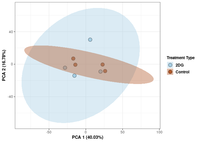
Scree plot and summary statistics hippocampus
tdata.FPKM.sample.info <- readRDS(here("Data","20190406_RNAseq_B6_4wk_2DG_counts_phenotypes.RData"))

tdata.FPKM.sample.info.hippocampus <- rownames_to_column(tdata.FPKM.sample.info) %>% filter(Tissue=="Hippocampus" & Time=="4 wks") %>% column_to_rownames('rowname')

tdata.FPKM <- readRDS(here("Data","20190406_RNAseq_B6_4wk_2DG_counts_numeric.RData"))

log.tdata.FPKM <- log(tdata.FPKM + 1)
log.tdata.FPKM <- as.data.frame(log.tdata.FPKM)

rows <- rownames(tdata.FPKM.sample.info.hippocampus)

log.tdata.FPKM.hippocampus <- rownames_to_column(log.tdata.FPKM)

log.tdata.FPKM.hippocampus <- log.tdata.FPKM.hippocampus %>% filter(rowname %in% rows) %>% column_to_rownames('rowname')

pca <- prcomp(log.tdata.FPKM.hippocampus, center = T)

screeplot(pca,type = "lines")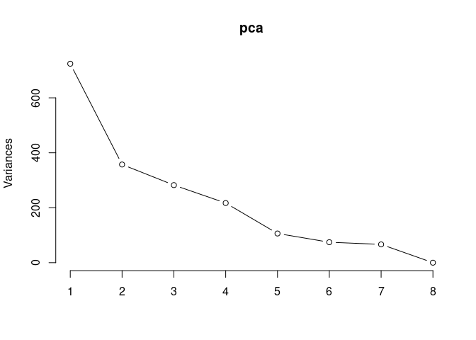
summary(pca)## Importance of components:
## PC1 PC2 PC3 PC4 PC5 PC6 PC7
## Standard deviation 26.9090 18.9018 16.8026 14.7323 10.3058 8.62958 8.1568
## Proportion of Variance 0.3961 0.1955 0.1545 0.1187 0.0581 0.04074 0.0364
## Cumulative Proportion 0.3961 0.5916 0.7460 0.8648 0.9229 0.96360 1.0000
## PC8
## Standard deviation 1.722e-14
## Proportion of Variance 0.000e+00
## Cumulative Proportion 1.000e+00Treatment hippocampus
Treatment_color <- as.factor(tdata.FPKM.sample.info.hippocampus$Treatment)
Treatment_color <- as.data.frame(Treatment_color)
col_treatment <- colorRampPalette(brewer.pal(n = 12, name = "Paired"))(2)[Treatment_color$Treatment_color]
pca_treatment <- cbind(Treatment_color,pca$x[,1],pca$x[,2])
pca_treatment <- as.data.frame(pca_treatment)

p <- ggplot(pca_treatment,aes(pca$x[,1], pca$x[,2]))
p <- p + geom_point(aes(fill = as.factor(pca_treatment$Treatment_color)), shape=21, size=4) + theme_bw()
p <- p + theme(legend.title = element_text(size=10,face="bold")) +
  theme(legend.text = element_text(size=10, face="bold"))
p <- p + xlab("PCA 1 (39.61%)") + ylab("PCA 2 (19.55%)") + theme(axis.title = element_text(face="bold"))
p <- p + stat_ellipse(aes(pca$x[,1], pca$x[,2], group = Treatment_color, fill = as.factor(pca_treatment$Treatment_color)), geom="polygon",level=0.95,alpha=0.4) +
  scale_fill_manual(values=c("#A6CEE3", "#B15928"),name="Treatment Type",
                       breaks=c("2DG", "None"),
                       labels=c("2DG", "Control")) +
  scale_linetype_manual(values=c(1,2))
print(p)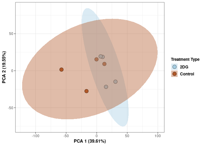
Scree plot and summary statistics liver
tdata.FPKM.sample.info <- readRDS(here("Data","20190406_RNAseq_B6_4wk_2DG_counts_phenotypes.RData"))

tdata.FPKM.sample.info.liver <- rownames_to_column(tdata.FPKM.sample.info) %>% filter(Tissue=="Liver" & Time=="4 wks") %>% column_to_rownames('rowname')

tdata.FPKM <- readRDS(here("Data","20190406_RNAseq_B6_4wk_2DG_counts_numeric.RData"))

log.tdata.FPKM <- log(tdata.FPKM + 1)
log.tdata.FPKM <- as.data.frame(log.tdata.FPKM)

rows <- rownames(tdata.FPKM.sample.info.liver)

log.tdata.FPKM.liver <- rownames_to_column(log.tdata.FPKM)

log.tdata.FPKM.liver <- log.tdata.FPKM.liver %>% filter(rowname %in% rows) %>% column_to_rownames('rowname')

pca <- prcomp(log.tdata.FPKM.liver, center = T)

screeplot(pca,type = "lines")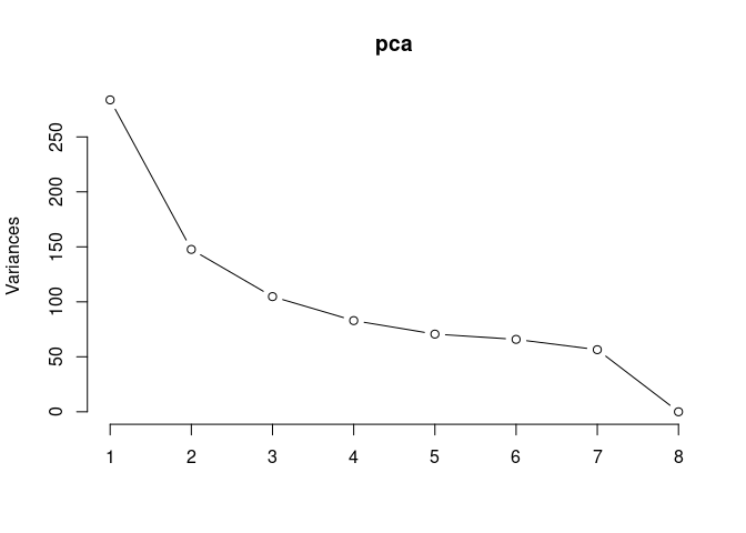
summary(pca)## Importance of components:
## PC1 PC2 PC3 PC4 PC5 PC6 PC7
## Standard deviation 16.8416 12.1513 10.2341 9.1064 8.4045 8.1147 7.51521
## Proportion of Variance 0.3493 0.1819 0.1290 0.1021 0.0870 0.0811 0.06956
## Cumulative Proportion 0.3493 0.5312 0.6602 0.7623 0.8493 0.9304 1.00000
## PC8
## Standard deviation 1.454e-14
## Proportion of Variance 0.000e+00
## Cumulative Proportion 1.000e+00Treatment liver
Treatment_color <- as.factor(tdata.FPKM.sample.info.liver$Treatment)
Treatment_color <- as.data.frame(Treatment_color)
col_treatment <- colorRampPalette(brewer.pal(n = 12, name = "Paired"))(2)[Treatment_color$Treatment_color]
pca_treatment <- cbind(Treatment_color,pca$x[,1],pca$x[,2])
pca_treatment <- as.data.frame(pca_treatment)

p <- ggplot(pca_treatment,aes(pca$x[,1], pca$x[,2]))
p <- p + geom_point(aes(fill = as.factor(pca_treatment$Treatment_color)), shape=21, size=4) + theme_bw()
p <- p + theme(legend.title = element_text(size=10,face="bold")) +
  theme(legend.text = element_text(size=10, face="bold"))
p <- p + xlab("PCA 1 (34.93%)") + ylab("PCA 2 (18.19%)") + theme(axis.title = element_text(face="bold"))
p <- p + stat_ellipse(aes(pca$x[,1], pca$x[,2], group = Treatment_color, fill = as.factor(pca_treatment$Treatment_color)), geom="polygon",level=0.95,alpha=0.4) +
  scale_fill_manual(values=c("#A6CEE3", "#B15928"),name="Treatment Type",
                       breaks=c("2DG", "None"),
                       labels=c("2DG", "Control")) +
  scale_linetype_manual(values=c(1,2))
print(p)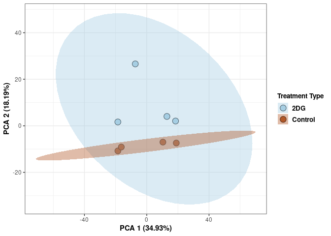
Scree plot and summary statistics heart
tdata.FPKM.sample.info <- readRDS(here("Data","20190406_RNAseq_B6_4wk_2DG_counts_phenotypes.RData"))

tdata.FPKM.sample.info.heart <- rownames_to_column(tdata.FPKM.sample.info) %>% filter(Tissue=="Heart" & Time=="4 wks") %>% column_to_rownames('rowname')

tdata.FPKM <- readRDS(here("Data","20190406_RNAseq_B6_4wk_2DG_counts_numeric.RData"))

log.tdata.FPKM <- log(tdata.FPKM + 1)
log.tdata.FPKM <- as.data.frame(log.tdata.FPKM)

rows <- rownames(tdata.FPKM.sample.info.heart)

log.tdata.FPKM.heart <- rownames_to_column(log.tdata.FPKM)

log.tdata.FPKM.heart <- log.tdata.FPKM.heart %>% filter(rowname %in% rows) %>% column_to_rownames('rowname')

pca <- prcomp(log.tdata.FPKM.heart, center = T)

screeplot(pca,type = "lines")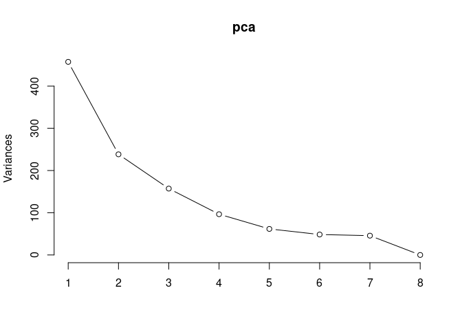
summary(pca)## Importance of components:
## PC1 PC2 PC3 PC4 PC5 PC6 PC7
## Standard deviation 21.3855 15.4393 12.5372 9.82365 7.8528 6.95813 6.76139
## Proportion of Variance 0.4138 0.2157 0.1422 0.08732 0.0558 0.04381 0.04137
## Cumulative Proportion 0.4138 0.6295 0.7717 0.85903 0.9148 0.95863 1.00000
## PC8
## Standard deviation 1.397e-14
## Proportion of Variance 0.000e+00
## Cumulative Proportion 1.000e+00Treatment heart
Treatment_color <- as.factor(tdata.FPKM.sample.info.heart$Treatment)
Treatment_color <- as.data.frame(Treatment_color)
col_treatment <- colorRampPalette(brewer.pal(n = 12, name = "Paired"))(2)[Treatment_color$Treatment_color]
pca_treatment <- cbind(Treatment_color,pca$x[,1],pca$x[,2])
pca_treatment <- as.data.frame(pca_treatment)

p <- ggplot(pca_treatment,aes(pca$x[,1], pca$x[,2]))
p <- p + geom_point(aes(fill = as.factor(pca_treatment$Treatment_color)), shape=21, size=4) + theme_bw()
p <- p + theme(legend.title = element_text(size=10,face="bold")) +
  theme(legend.text = element_text(size=10, face="bold"))
p <- p + xlab("PCA 1 (41.38%)") + ylab("PCA 2 (21.57%)") + theme(axis.title = element_text(face="bold"))
p <- p + stat_ellipse(aes(pca$x[,1], pca$x[,2], group = Treatment_color, fill = as.factor(pca_treatment$Treatment_color)), geom="polygon",level=0.95,alpha=0.4) +
  scale_fill_manual(values=c("#A6CEE3", "#B15928"),name="Treatment Type",
                       breaks=c("2DG", "None"),
                       labels=c("2DG", "Control")) +
  scale_linetype_manual(values=c(1,2))
print(p)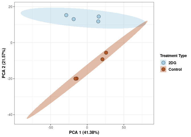
Scree plot and summary statistics small intestine
tdata.FPKM.sample.info <- readRDS(here("Data","20190406_RNAseq_B6_4wk_2DG_counts_phenotypes.RData"))

tdata.FPKM.sample.info.small.intestine <- rownames_to_column(tdata.FPKM.sample.info) %>% filter(Tissue=="Small Intestine" & Time=="4 wks") %>% column_to_rownames('rowname')

tdata.FPKM <- readRDS(here("Data","20190406_RNAseq_B6_4wk_2DG_counts_numeric.RData"))

log.tdata.FPKM <- log(tdata.FPKM + 1)
log.tdata.FPKM <- as.data.frame(log.tdata.FPKM)

rows <- rownames(tdata.FPKM.sample.info.small.intestine)

log.tdata.FPKM.small.intestine <- rownames_to_column(log.tdata.FPKM)

log.tdata.FPKM.small.intestine <- log.tdata.FPKM.small.intestine %>% filter(rowname %in% rows) %>% column_to_rownames('rowname')

pca <- prcomp(log.tdata.FPKM.small.intestine, center = T)

screeplot(pca,type = "lines")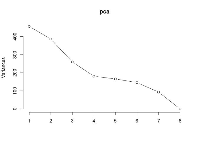
summary(pca)## Importance of components:
## PC1 PC2 PC3 PC4 PC5 PC6
## Standard deviation 21.3583 19.6585 16.1215 13.4519 12.87716 12.06583
## Proportion of Variance 0.2702 0.2289 0.1540 0.1072 0.09823 0.08624
## Cumulative Proportion 0.2702 0.4991 0.6531 0.7603 0.85852 0.94476
## PC7 PC8
## Standard deviation 9.65686 1.71e-14
## Proportion of Variance 0.05524 0.00e+00
## Cumulative Proportion 1.00000 1.00e+00Treatment small intestine
Treatment_color <- as.factor(tdata.FPKM.sample.info.small.intestine$Treatment)
Treatment_color <- as.data.frame(Treatment_color)
col_treatment <- colorRampPalette(brewer.pal(n = 12, name = "Paired"))(2)[Treatment_color$Treatment_color]
pca_treatment <- cbind(Treatment_color,pca$x[,1],pca$x[,2])
pca_treatment <- as.data.frame(pca_treatment)

p <- ggplot(pca_treatment,aes(pca$x[,1], pca$x[,2]))
p <- p + geom_point(aes(fill = as.factor(pca_treatment$Treatment_color)), shape=21, size=4) + theme_bw()
p <- p + theme(legend.title = element_text(size=10,face="bold")) +
  theme(legend.text = element_text(size=10, face="bold"))
p <- p + xlab("PCA 1 (27.02%)") + ylab("PCA 2 (22.89%)") + theme(axis.title = element_text(face="bold"))
p <- p + stat_ellipse(aes(pca$x[,1], pca$x[,2], group = Treatment_color, fill = as.factor(pca_treatment$Treatment_color)), geom="polygon",level=0.95,alpha=0.4) +
  scale_fill_manual(values=c("#A6CEE3", "#B15928"),name="Treatment Type",
                       breaks=c("2DG", "None"),
                       labels=c("2DG", "Control")) +
  scale_linetype_manual(values=c(1,2))
print(p)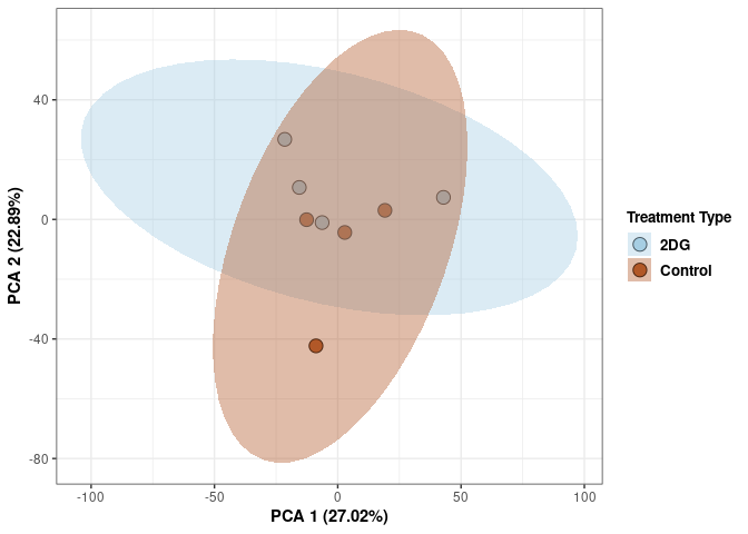
Scree plot and summary statistics skeletal muscle
tdata.FPKM.sample.info <- readRDS(here("Data","20190406_RNAseq_B6_4wk_2DG_counts_phenotypes.RData"))

tdata.FPKM.sample.info.skeletal.muscle <- rownames_to_column(tdata.FPKM.sample.info) %>% filter(Tissue=="Skeletal Muscle" & Time=="4 wks") %>% column_to_rownames('rowname')

tdata.FPKM <- readRDS(here("Data","20190406_RNAseq_B6_4wk_2DG_counts_numeric.RData"))

log.tdata.FPKM <- log(tdata.FPKM + 1)
log.tdata.FPKM <- as.data.frame(log.tdata.FPKM)

rows <- rownames(tdata.FPKM.sample.info.skeletal.muscle)

log.tdata.FPKM.skeletal.muscle <- rownames_to_column(log.tdata.FPKM)

log.tdata.FPKM.skeletal.muscle <- log.tdata.FPKM.skeletal.muscle %>% filter(rowname %in% rows) %>% column_to_rownames('rowname')

pca <- prcomp(log.tdata.FPKM.skeletal.muscle, center = T)

screeplot(pca,type = "lines")
summary(pca)## Importance of components:
## PC1 PC2 PC3 PC4 PC5 PC6
## Standard deviation 21.0792 18.0728 15.7698 11.6371 10.81314 10.17884
## Proportion of Variance 0.3071 0.2258 0.1719 0.0936 0.08081 0.07161
## Cumulative Proportion 0.3071 0.5329 0.7047 0.7983 0.87913 0.95074
## PC7 PC8
## Standard deviation 8.44197 1.358e-14
## Proportion of Variance 0.04926 0.000e+00
## Cumulative Proportion 1.00000 1.000e+00Treatment skeletal muscle
Treatment_color <- as.factor(tdata.FPKM.sample.info.skeletal.muscle$Treatment)
Treatment_color <- as.data.frame(Treatment_color)
col_treatment <- colorRampPalette(brewer.pal(n = 12, name = "Paired"))(2)[Treatment_color$Treatment_color]
pca_treatment <- cbind(Treatment_color,pca$x[,1],pca$x[,2])
pca_treatment <- as.data.frame(pca_treatment)

p <- ggplot(pca_treatment,aes(pca$x[,1], pca$x[,2]))
p <- p + geom_point(aes(fill = as.factor(pca_treatment$Treatment_color)), shape=21, size=4) + theme_bw()
p <- p + theme(legend.title = element_text(size=10,face="bold")) +
  theme(legend.text = element_text(size=10, face="bold"))
p <- p + xlab("PCA 1 (30.71%)") + ylab("PCA 2 (22.58%)") + theme(axis.title = element_text(face="bold"))
p <- p + stat_ellipse(aes(pca$x[,1], pca$x[,2], group = Treatment_color, fill = as.factor(pca_treatment$Treatment_color)), geom="polygon",level=0.95,alpha=0.4) +
  scale_fill_manual(values=c("#A6CEE3", "#B15928"),name="Treatment Type",
                       breaks=c("2DG", "None"),
                       labels=c("2DG", "Control")) +
  scale_linetype_manual(values=c(1,2))
print(p)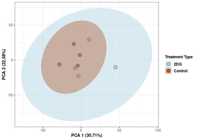
Scree plot and summary statistics prefrontal cortex
tdata.FPKM.sample.info <- readRDS(here("Data","20190406_RNAseq_B6_4wk_2DG_counts_phenotypes.RData"))

tdata.FPKM.sample.info.prefrontal.cortex <- rownames_to_column(tdata.FPKM.sample.info) %>% filter(Tissue=="Pre-frontal Cortex" & Time=="4 wks") %>% column_to_rownames('rowname')

tdata.FPKM <- readRDS(here("Data","20190406_RNAseq_B6_4wk_2DG_counts_numeric.RData"))

log.tdata.FPKM <- log(tdata.FPKM + 1)
log.tdata.FPKM <- as.data.frame(log.tdata.FPKM)

rows <- rownames(tdata.FPKM.sample.info.prefrontal.cortex)

log.tdata.FPKM.prefrontal.cortex <- rownames_to_column(log.tdata.FPKM)

log.tdata.FPKM.prefrontal.cortex <- log.tdata.FPKM.prefrontal.cortex %>% filter(rowname %in% rows) %>% column_to_rownames('rowname')

pca <- prcomp(log.tdata.FPKM.prefrontal.cortex, center = T)

screeplot(pca,type = "lines")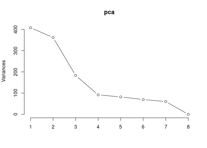
summary(pca)## Importance of components:
## PC1 PC2 PC3 PC4 PC5 PC6 PC7
## Standard deviation 20.1953 19.0225 13.5387 9.58331 9.05823 8.34644 7.7584
## Proportion of Variance 0.3245 0.2879 0.1459 0.07308 0.06529 0.05543 0.0479
## Cumulative Proportion 0.3245 0.6125 0.7583 0.83138 0.89667 0.95210 1.0000
## PC8
## Standard deviation 1.741e-14
## Proportion of Variance 0.000e+00
## Cumulative Proportion 1.000e+00Treatment prefrontal cortex
Treatment_color <- as.factor(tdata.FPKM.sample.info.prefrontal.cortex$Treatment)
Treatment_color <- as.data.frame(Treatment_color)
col_treatment <- colorRampPalette(brewer.pal(n = 12, name = "Paired"))(2)[Treatment_color$Treatment_color]
pca_treatment <- cbind(Treatment_color,pca$x[,1],pca$x[,2])
pca_treatment <- as.data.frame(pca_treatment)

p <- ggplot(pca_treatment,aes(pca$x[,1], pca$x[,2]))
p <- p + geom_point(aes(fill = as.factor(pca_treatment$Treatment_color)), shape=21, size=4) + theme_bw()
p <- p + theme(legend.title = element_text(size=10,face="bold")) +
  theme(legend.text = element_text(size=10, face="bold"))
p <- p + xlab("PCA 1 (32.45%)") + ylab("PCA 2 (28.79%)") + theme(axis.title = element_text(face="bold"))
p <- p + stat_ellipse(aes(pca$x[,1], pca$x[,2], group = Treatment_color, fill = as.factor(pca_treatment$Treatment_color)), geom="polygon",level=0.95,alpha=0.4) +
  scale_fill_manual(values=c("#A6CEE3", "#B15928"),name="Treatment Type",
                       breaks=c("2DG", "None"),
                       labels=c("2DG", "Control")) +
  scale_linetype_manual(values=c(1,2))
print(p)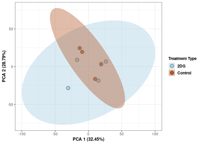
PCA (log Time by tissue 2DG)
These plots subset the data so each plot contains mice that were treated with 2DG for 96hrs or 4wks for each tissue.
Scree plot and summary statistics Spleen
tdata.FPKM.sample.info <- readRDS(here("Data","20190406_RNAseq_B6_4wk_2DG_counts_phenotypes.RData"))

tdata.FPKM.sample.info.spleen <- rownames_to_column(tdata.FPKM.sample.info) %>% filter(Tissue=="Spleen" & Treatment=="2DG") %>% column_to_rownames('rowname')

tdata.FPKM <- readRDS(here("Data","20190406_RNAseq_B6_4wk_2DG_counts_numeric.RData"))

log.tdata.FPKM <- log(tdata.FPKM + 1)
log.tdata.FPKM <- as.data.frame(log.tdata.FPKM)

rows <- rownames(tdata.FPKM.sample.info.spleen)

log.tdata.FPKM.spleen <- rownames_to_column(log.tdata.FPKM)

log.tdata.FPKM.spleen <- log.tdata.FPKM.spleen %>% filter(rowname %in% rows) %>% column_to_rownames('rowname')

pca <- prcomp(log.tdata.FPKM.spleen, center = T)

screeplot(pca,type = "lines")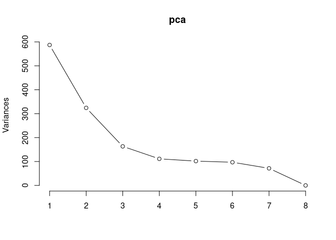
summary(pca)## Importance of components:
## PC1 PC2 PC3 PC4 PC5 PC6
## Standard deviation 24.2333 18.0077 12.7767 10.54248 10.08216 9.84557
## Proportion of Variance 0.4033 0.2227 0.1121 0.07634 0.06982 0.06658
## Cumulative Proportion 0.4033 0.6261 0.7382 0.81454 0.88436 0.95094
## PC7 PC8
## Standard deviation 8.45195 1.8e-14
## Proportion of Variance 0.04906 0.0e+00
## Cumulative Proportion 1.00000 1.0e+00Time spleen
Time_color <- as.factor(tdata.FPKM.sample.info.spleen$Time)
Time_color <- as.data.frame(Time_color)
col_time <- colorRampPalette(brewer.pal(n = 12, name = "Paired"))(2)[Time_color$Time_color]
pca_time <- cbind(Time_color,pca$x[,1],pca$x[,2])
pca_time <- as.data.frame(pca_time)

p <- ggplot(pca_time,aes(pca$x[,1], pca$x[,2]))
p <- p + geom_point(aes(fill = as.factor(pca_time$Time_color)), shape=21, size=4) + theme_bw()
p <- p + theme(legend.title = element_text(size=10,face="bold")) +
  theme(legend.text = element_text(size=10, face="bold"))
p <- p + xlab("PCA 1 (40.33%)") + ylab("PCA 2 (22.27%)") + theme(axis.title = element_text(face="bold"))
p <- p + stat_ellipse(aes(pca$x[,1], pca$x[,2], group = Time_color, fill = as.factor(pca_time$Time_color)), geom="polygon",level=0.95,alpha=0.4) +
  scale_fill_manual(values=c("#A6CEE3", "#B15928"),name="Time",
                       breaks=c("4 wks", "96 hrs"),
                       labels=c("4 wks", "96 hrs")) +
  scale_linetype_manual(values=c(1,2))
print(p)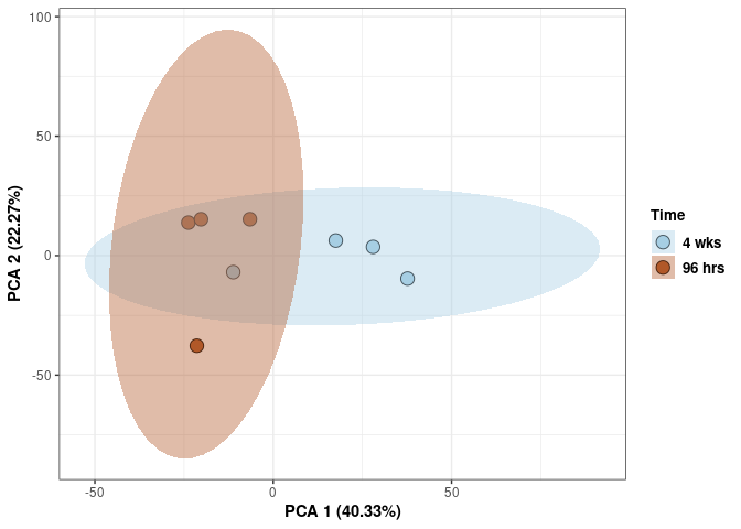
Scree plot and summary statistics kidney
tdata.FPKM.sample.info <- readRDS(here("Data","20190406_RNAseq_B6_4wk_2DG_counts_phenotypes.RData"))

tdata.FPKM.sample.info.kidney <- rownames_to_column(tdata.FPKM.sample.info) %>% filter(Tissue=="Kidney" & Treatment=="2DG") %>% column_to_rownames('rowname')

tdata.FPKM <- readRDS(here("Data","20190406_RNAseq_B6_4wk_2DG_counts_numeric.RData"))

log.tdata.FPKM <- log(tdata.FPKM + 1)
log.tdata.FPKM <- as.data.frame(log.tdata.FPKM)

rows <- rownames(tdata.FPKM.sample.info.kidney)

log.tdata.FPKM.kidney <- rownames_to_column(log.tdata.FPKM)

log.tdata.FPKM.kidney <- log.tdata.FPKM.kidney %>% filter(rowname %in% rows) %>% column_to_rownames('rowname')

pca <- prcomp(log.tdata.FPKM.kidney, center = T)

screeplot(pca,type = "lines")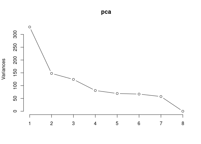
summary(pca)## Importance of components:
## PC1 PC2 PC3 PC4 PC5 PC6 PC7
## Standard deviation 18.1363 12.1508 11.1475 8.99836 8.32345 8.18849 7.57823
## Proportion of Variance 0.3757 0.1686 0.1419 0.09248 0.07913 0.07658 0.06559
## Cumulative Proportion 0.3757 0.5443 0.6862 0.77870 0.85783 0.93441 1.00000
## PC8
## Standard deviation 1.57e-14
## Proportion of Variance 0.00e+00
## Cumulative Proportion 1.00e+00Time kidney
Time_color <- as.factor(tdata.FPKM.sample.info.kidney$Time)
Time_color <- as.data.frame(Time_color)
col_time <- colorRampPalette(brewer.pal(n = 12, name = "Paired"))(2)[Time_color$Time_color]
pca_time <- cbind(Time_color,pca$x[,1],pca$x[,2])
pca_time <- as.data.frame(pca_time)

p <- ggplot(pca_time,aes(pca$x[,1], pca$x[,2]))
p <- p + geom_point(aes(fill = as.factor(pca_time$Time_color)), shape=21, size=4) + theme_bw()
p <- p + theme(legend.title = element_text(size=10,face="bold")) +
  theme(legend.text = element_text(size=10, face="bold"))
p <- p + xlab("PCA 1 (37.57%)") + ylab("PCA 2 (16.86%)") + theme(axis.title = element_text(face="bold"))
p <- p + stat_ellipse(aes(pca$x[,1], pca$x[,2], group = Time_color, fill = as.factor(pca_time$Time_color)), geom="polygon",level=0.95,alpha=0.4) +
  scale_fill_manual(values=c("#A6CEE3", "#B15928"),name="Time",
                       breaks=c("4 wks", "96 hrs"),
                       labels=c("4 wks", "96 hrs")) +
  scale_linetype_manual(values=c(1,2))
print(p)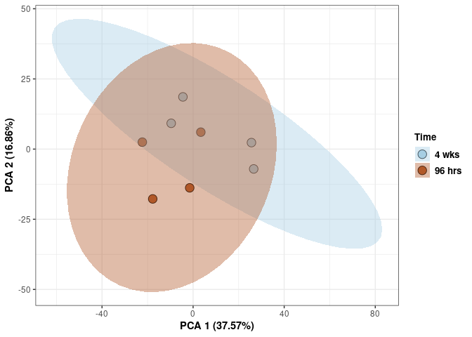
Scree plot and summary statistics hypothalamus
tdata.FPKM.sample.info <- readRDS(here("Data","20190406_RNAseq_B6_4wk_2DG_counts_phenotypes.RData"))

tdata.FPKM.sample.info.hypothalamus <- rownames_to_column(tdata.FPKM.sample.info) %>% filter(Tissue=="Hypothanamus" & Treatment=="2DG") %>% column_to_rownames('rowname')

tdata.FPKM <- readRDS(here("Data","20190406_RNAseq_B6_4wk_2DG_counts_numeric.RData"))

log.tdata.FPKM <- log(tdata.FPKM + 1)
log.tdata.FPKM <- as.data.frame(log.tdata.FPKM)

rows <- rownames(tdata.FPKM.sample.info.hypothalamus)

log.tdata.FPKM.hypothalamus <- rownames_to_column(log.tdata.FPKM)

log.tdata.FPKM.hypothalamus <- log.tdata.FPKM.hypothalamus %>% filter(rowname %in% rows) %>% column_to_rownames('rowname')

pca <- prcomp(log.tdata.FPKM.hypothalamus, center = T)

screeplot(pca,type = "lines")
summary(pca)## Importance of components:
## PC1 PC2 PC3 PC4 PC5 PC6 PC7
## Standard deviation 20.795 13.8274 11.7284 10.34150 9.32984 8.96316 7.69299
## Proportion of Variance 0.395 0.1746 0.1257 0.09769 0.07951 0.07339 0.05406
## Cumulative Proportion 0.395 0.5697 0.6953 0.79304 0.87255 0.94594 1.00000
## PC8
## Standard deviation 1.741e-14
## Proportion of Variance 0.000e+00
## Cumulative Proportion 1.000e+00Time hypothalamus
Time_color <- as.factor(tdata.FPKM.sample.info.hypothalamus$Time)
Time_color <- as.data.frame(Time_color)
col_time <- colorRampPalette(brewer.pal(n = 12, name = "Paired"))(2)[Time_color$Time_color]
pca_time <- cbind(Time_color,pca$x[,1],pca$x[,2])
pca_time <- as.data.frame(pca_time)

p <- ggplot(pca_time,aes(pca$x[,1], pca$x[,2]))
p <- p + geom_point(aes(fill = as.factor(pca_time$Time_color)), shape=21, size=4) + theme_bw()
p <- p + theme(legend.title = element_text(size=10,face="bold")) +
  theme(legend.text = element_text(size=10, face="bold"))
p <- p + xlab("PCA 1 (39.5%)") + ylab("PCA 2 (17.46%)") + theme(axis.title = element_text(face="bold"))
p <- p + stat_ellipse(aes(pca$x[,1], pca$x[,2], group = Time_color, fill = as.factor(pca_time$Time_color)), geom="polygon",level=0.95,alpha=0.4) +
  scale_fill_manual(values=c("#A6CEE3", "#B15928"),name="Time",
                       breaks=c("4 wks", "96 hrs"),
                       labels=c("4 wks", "96 hrs")) +
  scale_linetype_manual(values=c(1,2))
print(p)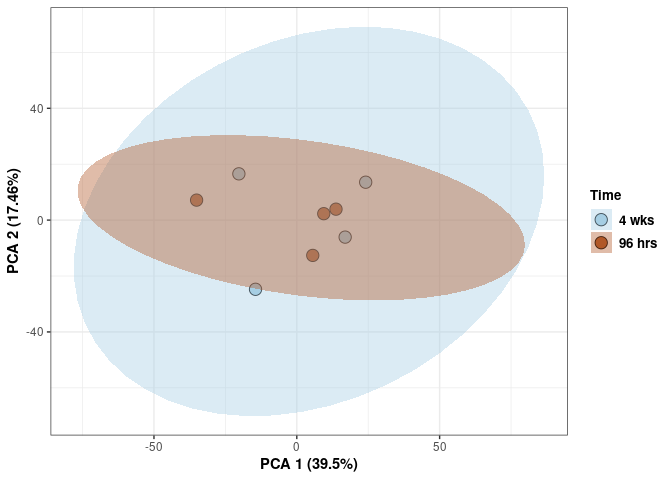
Scree plot and summary statistics hippocampus
tdata.FPKM.sample.info <- readRDS(here("Data","20190406_RNAseq_B6_4wk_2DG_counts_phenotypes.RData"))

tdata.FPKM.sample.info.hippocampus <- rownames_to_column(tdata.FPKM.sample.info) %>% filter(Tissue=="Hippocampus" & Treatment=="2DG") %>% column_to_rownames('rowname')

tdata.FPKM <- readRDS(here("Data","20190406_RNAseq_B6_4wk_2DG_counts_numeric.RData"))

log.tdata.FPKM <- log(tdata.FPKM + 1)
log.tdata.FPKM <- as.data.frame(log.tdata.FPKM)

rows <- rownames(tdata.FPKM.sample.info.hippocampus)

log.tdata.FPKM.hippocampus <- rownames_to_column(log.tdata.FPKM)

log.tdata.FPKM.hippocampus <- log.tdata.FPKM.hippocampus %>% filter(rowname %in% rows) %>% column_to_rownames('rowname')

pca <- prcomp(log.tdata.FPKM.hippocampus, center = T)

screeplot(pca,type = "lines")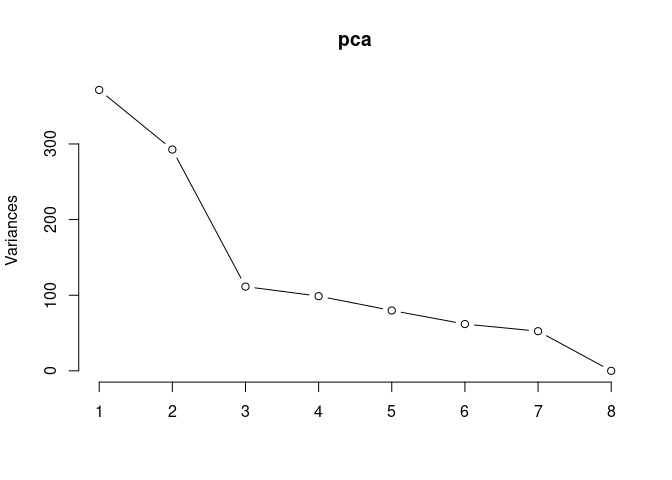
summary(pca)## Importance of components:
## PC1 PC2 PC3 PC4 PC5 PC6 PC7
## Standard deviation 19.2717 17.1060 10.5540 9.93822 8.93221 7.86410 7.24082
## Proportion of Variance 0.3477 0.2739 0.1043 0.09246 0.07469 0.05789 0.04908
## Cumulative Proportion 0.3477 0.6216 0.7259 0.81834 0.89302 0.95092 1.00000
## PC8
## Standard deviation 1.708e-14
## Proportion of Variance 0.000e+00
## Cumulative Proportion 1.000e+00Time hippocampus
Time_color <- as.factor(tdata.FPKM.sample.info.hippocampus$Time)
Time_color <- as.data.frame(Time_color)
col_time <- colorRampPalette(brewer.pal(n = 12, name = "Paired"))(2)[Time_color$Time_color]
pca_time <- cbind(Time_color,pca$x[,1],pca$x[,2])
pca_time <- as.data.frame(pca_time)

p <- ggplot(pca_time,aes(pca$x[,1], pca$x[,2]))
p <- p + geom_point(aes(fill = as.factor(pca_time$Time_color)), shape=21, size=4) + theme_bw()
p <- p + theme(legend.title = element_text(size=10,face="bold")) +
  theme(legend.text = element_text(size=10, face="bold"))
p <- p + xlab("PCA 1 (34.77%)") + ylab("PCA 2 (27.39%)") + theme(axis.title = element_text(face="bold"))
p <- p + stat_ellipse(aes(pca$x[,1], pca$x[,2], group = Time_color, fill = as.factor(pca_time$Time_color)), geom="polygon",level=0.95,alpha=0.4) +
  scale_fill_manual(values=c("#A6CEE3", "#B15928"),name="Time",
                       breaks=c("4 wks", "96 hrs"),
                       labels=c("4 wks", "96 hrs")) +
  scale_linetype_manual(values=c(1,2))
print(p)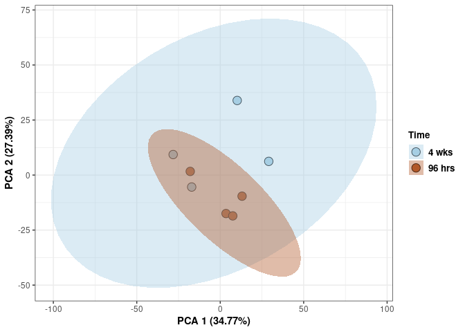
Scree plot and summary statistics liver
tdata.FPKM.sample.info <- readRDS(here("Data","20190406_RNAseq_B6_4wk_2DG_counts_phenotypes.RData"))

tdata.FPKM.sample.info.liver <- rownames_to_column(tdata.FPKM.sample.info) %>% filter(Tissue=="Liver" & Treatment=="2DG") %>% column_to_rownames('rowname')

tdata.FPKM <- readRDS(here("Data","20190406_RNAseq_B6_4wk_2DG_counts_numeric.RData"))

log.tdata.FPKM <- log(tdata.FPKM + 1)
log.tdata.FPKM <- as.data.frame(log.tdata.FPKM)

rows <- rownames(tdata.FPKM.sample.info.liver)

log.tdata.FPKM.liver <- rownames_to_column(log.tdata.FPKM)

log.tdata.FPKM.liver <- log.tdata.FPKM.liver %>% filter(rowname %in% rows) %>% column_to_rownames('rowname')

pca <- prcomp(log.tdata.FPKM.liver, center = T)

screeplot(pca,type = "lines")
summary(pca)## Importance of components:
## PC1 PC2 PC3 PC4 PC5 PC6 PC7
## Standard deviation 17.9069 12.0897 10.3726 9.8132 8.77321 8.04748 7.49335
## Proportion of Variance 0.3692 0.1683 0.1239 0.1109 0.08861 0.07456 0.06465
## Cumulative Proportion 0.3692 0.5374 0.6613 0.7722 0.86079 0.93535 1.00000
## PC8
## Standard deviation 1.417e-14
## Proportion of Variance 0.000e+00
## Cumulative Proportion 1.000e+00Time liver
Time_color <- as.factor(tdata.FPKM.sample.info.liver$Time)
Time_color <- as.data.frame(Time_color)
col_time <- colorRampPalette(brewer.pal(n = 12, name = "Paired"))(2)[Time_color$Time_color]
pca_time <- cbind(Time_color,pca$x[,1],pca$x[,2])
pca_time <- as.data.frame(pca_time)

p <- ggplot(pca_time,aes(pca$x[,1], pca$x[,2]))
p <- p + geom_point(aes(fill = as.factor(pca_time$Time_color)), shape=21, size=4) + theme_bw()
p <- p + theme(legend.title = element_text(size=10,face="bold")) +
  theme(legend.text = element_text(size=10, face="bold"))
p <- p + xlab("PCA 1 (36.92%)") + ylab("PCA 2 (16.83%)") + theme(axis.title = element_text(face="bold"))
p <- p + stat_ellipse(aes(pca$x[,1], pca$x[,2], group = Time_color, fill = as.factor(pca_time$Time_color)), geom="polygon",level=0.95,alpha=0.4) +
  scale_fill_manual(values=c("#A6CEE3", "#B15928"),name="Time",
                       breaks=c("4 wks", "96 hrs"),
                       labels=c("4 wks", "96 hrs")) +
  scale_linetype_manual(values=c(1,2))
print(p)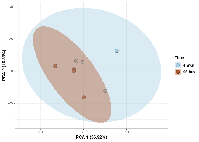
Scree plot and summary statistics heart
tdata.FPKM.sample.info <- readRDS(here("Data","20190406_RNAseq_B6_4wk_2DG_counts_phenotypes.RData"))

tdata.FPKM.sample.info.heart <- rownames_to_column(tdata.FPKM.sample.info) %>% filter(Tissue=="Heart" & Treatment=="2DG") %>% column_to_rownames('rowname')

tdata.FPKM <- readRDS(here("Data","20190406_RNAseq_B6_4wk_2DG_counts_numeric.RData"))

log.tdata.FPKM <- log(tdata.FPKM + 1)
log.tdata.FPKM <- as.data.frame(log.tdata.FPKM)

rows <- rownames(tdata.FPKM.sample.info.heart)

log.tdata.FPKM.heart <- rownames_to_column(log.tdata.FPKM)

log.tdata.FPKM.heart <- log.tdata.FPKM.heart %>% filter(rowname %in% rows) %>% column_to_rownames('rowname')

pca <- prcomp(log.tdata.FPKM.heart, center = T)

screeplot(pca,type = "lines")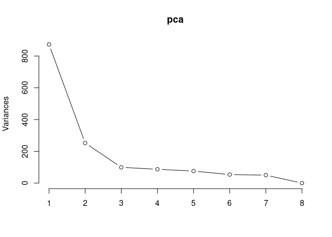
summary(pca)## Importance of components:
## PC1 PC2 PC3 PC4 PC5 PC6 PC7
## Standard deviation 29.5454 15.8880 9.96463 9.32495 8.70188 7.32929 7.08075
## Proportion of Variance 0.5854 0.1693 0.06659 0.05831 0.05078 0.03602 0.03362
## Cumulative Proportion 0.5854 0.7547 0.82126 0.87957 0.93035 0.96638 1.00000
## PC8
## Standard deviation 1.328e-14
## Proportion of Variance 0.000e+00
## Cumulative Proportion 1.000e+00Time heart
Time_color <- as.factor(tdata.FPKM.sample.info.heart$Time)
Time_color <- as.data.frame(Time_color)
col_time <- colorRampPalette(brewer.pal(n = 12, name = "Paired"))(2)[Time_color$Time_color]
pca_time <- cbind(Time_color,pca$x[,1],pca$x[,2])
pca_time <- as.data.frame(pca_time)

p <- ggplot(pca_time,aes(pca$x[,1], pca$x[,2]))
p <- p + geom_point(aes(fill = as.factor(pca_time$Time_color)), shape=21, size=4) + theme_bw()
p <- p + theme(legend.title = element_text(size=10,face="bold")) +
  theme(legend.text = element_text(size=10, face="bold"))
p <- p + xlab("PCA 1 (58.54%)") + ylab("PCA 2 (16.93%)") + theme(axis.title = element_text(face="bold"))
p <- p + stat_ellipse(aes(pca$x[,1], pca$x[,2], group = Time_color, fill = as.factor(pca_time$Time_color)), geom="polygon",level=0.95,alpha=0.4) +
  scale_fill_manual(values=c("#A6CEE3", "#B15928"),name="Time",
                       breaks=c("4 wks", "96 hrs"),
                       labels=c("4 wks", "96 hrs")) +
  scale_linetype_manual(values=c(1,2))
print(p)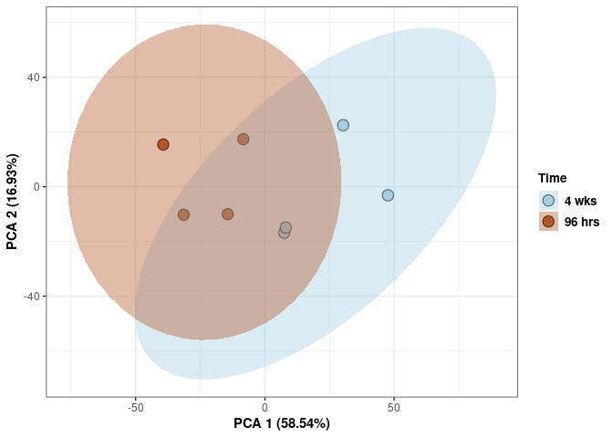
Scree plot and summary statistics small intestine
tdata.FPKM.sample.info <- readRDS(here("Data","20190406_RNAseq_B6_4wk_2DG_counts_phenotypes.RData"))

tdata.FPKM.sample.info.small.intestine <- rownames_to_column(tdata.FPKM.sample.info) %>% filter(Tissue=="Small Intestine" & Treatment=="2DG") %>% column_to_rownames('rowname')

tdata.FPKM <- readRDS(here("Data","20190406_RNAseq_B6_4wk_2DG_counts_numeric.RData"))

log.tdata.FPKM <- log(tdata.FPKM + 1)
log.tdata.FPKM <- as.data.frame(log.tdata.FPKM)

rows <- rownames(tdata.FPKM.sample.info.small.intestine)

log.tdata.FPKM.small.intestine <- rownames_to_column(log.tdata.FPKM)

log.tdata.FPKM.small.intestine <- log.tdata.FPKM.small.intestine %>% filter(rowname %in% rows) %>% column_to_rownames('rowname')

pca <- prcomp(log.tdata.FPKM.small.intestine, center = T)

screeplot(pca,type = "lines")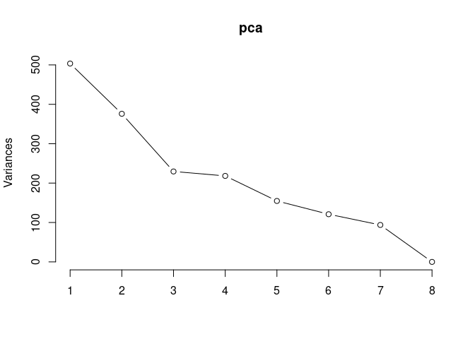
summary(pca)## Importance of components:
## PC1 PC2 PC3 PC4 PC5 PC6
## Standard deviation 22.4378 19.3889 15.1502 14.7740 12.43747 10.99986
## Proportion of Variance 0.2967 0.2216 0.1353 0.1286 0.09117 0.07132
## Cumulative Proportion 0.2967 0.5183 0.6536 0.7822 0.87341 0.94473
## PC7 PC8
## Standard deviation 9.68391 1.7e-14
## Proportion of Variance 0.05527 0.0e+00
## Cumulative Proportion 1.00000 1.0e+00Time small intestine
Time_color <- as.factor(tdata.FPKM.sample.info.small.intestine$Time)
Time_color <- as.data.frame(Time_color)
col_time <- colorRampPalette(brewer.pal(n = 12, name = "Paired"))(2)[Time_color$Time_color]
pca_time <- cbind(Time_color,pca$x[,1],pca$x[,2])
pca_time <- as.data.frame(pca_time)

p <- ggplot(pca_time,aes(pca$x[,1], pca$x[,2]))
p <- p + geom_point(aes(fill = as.factor(pca_time$Time_color)), shape=21, size=4) + theme_bw()
p <- p + theme(legend.title = element_text(size=10,face="bold")) +
  theme(legend.text = element_text(size=10, face="bold"))
p <- p + xlab("PCA 1 (29.67%)") + ylab("PCA 2 (22.16%)") + theme(axis.title = element_text(face="bold"))
p <- p + stat_ellipse(aes(pca$x[,1], pca$x[,2], group = Time_color, fill = as.factor(pca_time$Time_color)), geom="polygon",level=0.95,alpha=0.4) +
  scale_fill_manual(values=c("#A6CEE3", "#B15928"),name="Time",
                       breaks=c("4 wks", "96 hrs"),
                       labels=c("4 wks", "96 hrs")) +
  scale_linetype_manual(values=c(1,2))
print(p)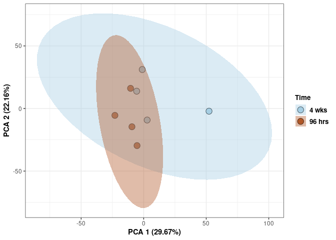
Scree plot and summary statistics skeletal muscle
tdata.FPKM.sample.info <- readRDS(here("Data","20190406_RNAseq_B6_4wk_2DG_counts_phenotypes.RData"))

tdata.FPKM.sample.info.skeletal.muscle <- rownames_to_column(tdata.FPKM.sample.info) %>% filter(Tissue=="Skeletal Muscle" & Treatment=="2DG") %>% column_to_rownames('rowname')

tdata.FPKM <- readRDS(here("Data","20190406_RNAseq_B6_4wk_2DG_counts_numeric.RData"))

log.tdata.FPKM <- log(tdata.FPKM + 1)
log.tdata.FPKM <- as.data.frame(log.tdata.FPKM)

rows <- rownames(tdata.FPKM.sample.info.skeletal.muscle)

log.tdata.FPKM.skeletal.muscle <- rownames_to_column(log.tdata.FPKM)

log.tdata.FPKM.skeletal.muscle <- log.tdata.FPKM.skeletal.muscle %>% filter(rowname %in% rows) %>% column_to_rownames('rowname')

pca <- prcomp(log.tdata.FPKM.skeletal.muscle, center = T)

screeplot(pca,type = "lines")
summary(pca)## Importance of components:
## PC1 PC2 PC3 PC4 PC5 PC6
## Standard deviation 25.4103 17.4812 14.9438 10.96355 10.61229 9.45465
## Proportion of Variance 0.4124 0.1952 0.1426 0.07676 0.07192 0.05709
## Cumulative Proportion 0.4124 0.6075 0.7501 0.82691 0.89884 0.95592
## PC7 PC8
## Standard deviation 8.30752 1.388e-14
## Proportion of Variance 0.04408 0.000e+00
## Cumulative Proportion 1.00000 1.000e+00Time skeletal muscle
Time_color <- as.factor(tdata.FPKM.sample.info.skeletal.muscle$Time)
Time_color <- as.data.frame(Time_color)
col_time <- colorRampPalette(brewer.pal(n = 12, name = "Paired"))(2)[Time_color$Time_color]
pca_time <- cbind(Time_color,pca$x[,1],pca$x[,2])
pca_time <- as.data.frame(pca_time)

p <- ggplot(pca_time,aes(pca$x[,1], pca$x[,2]))
p <- p + geom_point(aes(fill = as.factor(pca_time$Time_color)), shape=21, size=4) + theme_bw()
p <- p + theme(legend.title = element_text(size=10,face="bold")) +
  theme(legend.text = element_text(size=10, face="bold"))
p <- p + xlab("PCA 1 (41.24%)") + ylab("PCA 2 (19.52%)") + theme(axis.title = element_text(face="bold"))
p <- p + stat_ellipse(aes(pca$x[,1], pca$x[,2], group = Time_color, fill = as.factor(pca_time$Time_color)), geom="polygon",level=0.95,alpha=0.4) +
  scale_fill_manual(values=c("#A6CEE3", "#B15928"),name="Time",
                       breaks=c("4 wks", "96 hrs"),
                       labels=c("4 wks", "96 hrs")) +
  scale_linetype_manual(values=c(1,2))
print(p)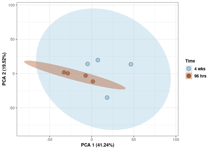
Scree plot and summary statistics prefrontal cortex
tdata.FPKM.sample.info <- readRDS(here("Data","20190406_RNAseq_B6_4wk_2DG_counts_phenotypes.RData"))

tdata.FPKM.sample.info.prefrontal.cortex <- rownames_to_column(tdata.FPKM.sample.info) %>% filter(Tissue=="Pre-frontal Cortex" & Treatment=="2DG") %>% column_to_rownames('rowname')

tdata.FPKM <- readRDS(here("Data","20190406_RNAseq_B6_4wk_2DG_counts_numeric.RData"))

log.tdata.FPKM <- log(tdata.FPKM + 1)
log.tdata.FPKM <- as.data.frame(log.tdata.FPKM)

rows <- rownames(tdata.FPKM.sample.info.prefrontal.cortex)

log.tdata.FPKM.prefrontal.cortex <- rownames_to_column(log.tdata.FPKM)

log.tdata.FPKM.prefrontal.cortex <- log.tdata.FPKM.prefrontal.cortex %>% filter(rowname %in% rows) %>% column_to_rownames('rowname')

pca <- prcomp(log.tdata.FPKM.prefrontal.cortex, center = T)

screeplot(pca,type = "lines")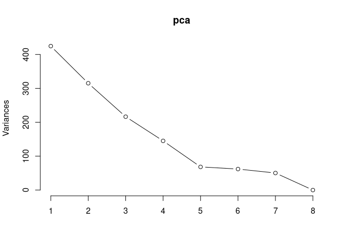
summary(pca)## Importance of components:
## PC1 PC2 PC3 PC4 PC5 PC6 PC7
## Standard deviation 20.6079 17.7520 14.7106 12.0443 8.26537 7.87287 7.09151
## Proportion of Variance 0.3313 0.2458 0.1688 0.1132 0.05329 0.04835 0.03923
## Cumulative Proportion 0.3313 0.5771 0.7460 0.8591 0.91242 0.96077 1.00000
## PC8
## Standard deviation 1.717e-14
## Proportion of Variance 0.000e+00
## Cumulative Proportion 1.000e+00Time prefrontal cortex
Time_color <- as.factor(tdata.FPKM.sample.info.prefrontal.cortex$Time)
Time_color <- as.data.frame(Time_color)
col_time <- colorRampPalette(brewer.pal(n = 12, name = "Paired"))(2)[Time_color$Time_color]
pca_time <- cbind(Time_color,pca$x[,1],pca$x[,2])
pca_time <- as.data.frame(pca_time)

p <- ggplot(pca_time,aes(pca$x[,1], pca$x[,2]))
p <- p + geom_point(aes(fill = as.factor(pca_time$Time_color)), shape=21, size=4) + theme_bw()
p <- p + theme(legend.title = element_text(size=10,face="bold")) +
  theme(legend.text = element_text(size=10, face="bold"))
p <- p + xlab("PCA 1 (33.13%)") + ylab("PCA 2 (24.58%)") + theme(axis.title = element_text(face="bold"))
p <- p + stat_ellipse(aes(pca$x[,1], pca$x[,2], group = Time_color, fill = as.factor(pca_time$Time_color)), geom="polygon",level=0.95,alpha=0.4) +
  scale_fill_manual(values=c("#A6CEE3", "#B15928"),name="Time",
                       breaks=c("4 wks", "96 hrs"),
                       labels=c("4 wks", "96 hrs")) +
  scale_linetype_manual(values=c(1,2))
print(p)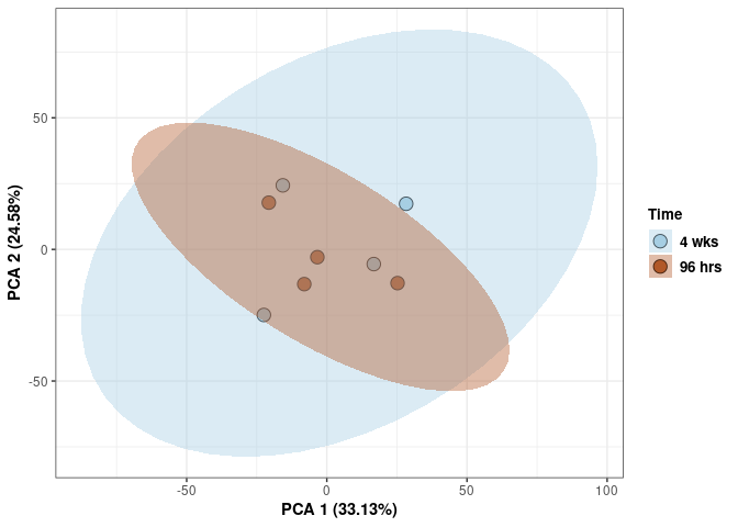
PCA (log Time by tissue control)
These plots subset the data so each plot contains mice that were treated with nothing for 96hrs or 4wks for each tissue.
Scree plot and summary statistics Spleen
tdata.FPKM.sample.info <- readRDS(here("Data","20190406_RNAseq_B6_4wk_2DG_counts_phenotypes.RData"))

tdata.FPKM.sample.info.spleen <- rownames_to_column(tdata.FPKM.sample.info) %>% filter(Tissue=="Spleen" & Treatment=="None") %>% column_to_rownames('rowname')

tdata.FPKM <- readRDS(here("Data","20190406_RNAseq_B6_4wk_2DG_counts_numeric.RData"))

log.tdata.FPKM <- log(tdata.FPKM + 1)
log.tdata.FPKM <- as.data.frame(log.tdata.FPKM)

rows <- rownames(tdata.FPKM.sample.info.spleen)

log.tdata.FPKM.spleen <- rownames_to_column(log.tdata.FPKM)

log.tdata.FPKM.spleen <- log.tdata.FPKM.spleen %>% filter(rowname %in% rows) %>% column_to_rownames('rowname')

pca <- prcomp(log.tdata.FPKM.spleen, center = T)

screeplot(pca,type = "lines")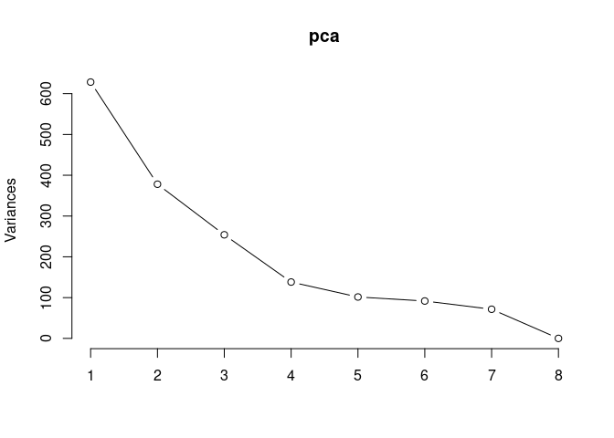
summary(pca)## Importance of components:
## PC1 PC2 PC3 PC4 PC5 PC6
## Standard deviation 25.0673 19.4419 15.9373 11.75291 10.07542 9.57413
## Proportion of Variance 0.3778 0.2273 0.1527 0.08306 0.06104 0.05512
## Cumulative Proportion 0.3778 0.6051 0.7578 0.84088 0.90192 0.95703
## PC7 PC8
## Standard deviation 8.45319 1.81e-14
## Proportion of Variance 0.04297 0.00e+00
## Cumulative Proportion 1.00000 1.00e+00Time spleen
Time_color <- as.factor(tdata.FPKM.sample.info.spleen$Time)
Time_color <- as.data.frame(Time_color)
col_time <- colorRampPalette(brewer.pal(n = 12, name = "Paired"))(2)[Time_color$Time_color]
pca_time <- cbind(Time_color,pca$x[,1],pca$x[,2])
pca_time <- as.data.frame(pca_time)

p <- ggplot(pca_time,aes(pca$x[,1], pca$x[,2]))
p <- p + geom_point(aes(fill = as.factor(pca_time$Time_color)), shape=21, size=4) + theme_bw()
p <- p + theme(legend.title = element_text(size=10,face="bold")) +
  theme(legend.text = element_text(size=10, face="bold"))
p <- p + xlab("PCA 1 (38.53%)") + ylab("PCA 2 (19.94%)") + theme(axis.title = element_text(face="bold"))
p <- p + stat_ellipse(aes(pca$x[,1], pca$x[,2], group = Time_color, fill = as.factor(pca_time$Time_color)), geom="polygon",level=0.95,alpha=0.4) +
  scale_fill_manual(values=c("#A6CEE3", "#B15928"),name="Time",
                       breaks=c("4 wks", "96 hrs"),
                       labels=c("4 wks", "96 hrs")) +
  scale_linetype_manual(values=c(1,2))
print(p)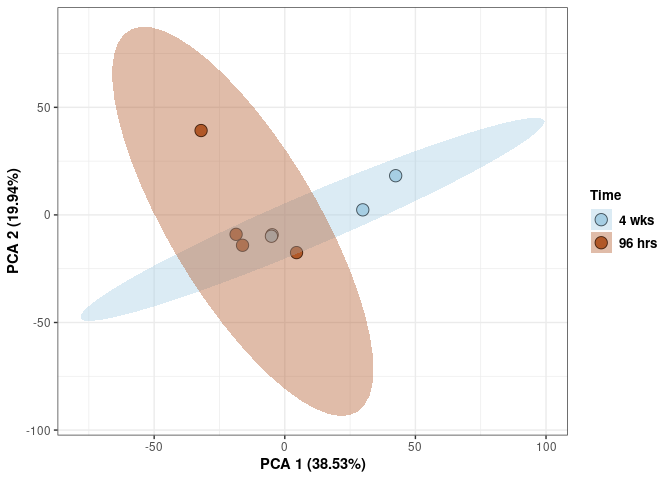
Scree plot and summary statistics kidney
tdata.FPKM.sample.info <- readRDS(here("Data","20190406_RNAseq_B6_4wk_2DG_counts_phenotypes.RData"))
tdata.FPKM.sample.info.kidney <- rownames_to_column(tdata.FPKM.sample.info) %>% filter(Tissue=="Kidney" & Treatment=="None") %>% column_to_rownames('rowname')
tdata.FPKM <- readRDS(here("Data","20190406_RNAseq_B6_4wk_2DG_counts_numeric.RData"))
log.tdata.FPKM <- log(tdata.FPKM + 1)
log.tdata.FPKM <- as.data.frame(log.tdata.FPKM)
rows <- rownames(tdata.FPKM.sample.info.kidney)
log.tdata.FPKM.kidney <- rownames_to_column(log.tdata.FPKM)
log.tdata.FPKM.kidney <- log.tdata.FPKM.kidney %>% filter(rowname %in% rows) %>% column_to_rownames('rowname')
pca <- prcomp(log.tdata.FPKM.kidney, center = T)
screeplot(pca,type = "lines")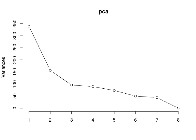
summary(pca)## Importance of components:
## PC1 PC2 PC3 PC4 PC5 PC6 PC7
## Standard deviation 18.4149 12.4984 9.7817 9.4459 8.54958 7.05922 6.62923
## Proportion of Variance 0.4003 0.1844 0.1129 0.1053 0.08629 0.05883 0.05188
## Cumulative Proportion 0.4003 0.5847 0.6977 0.8030 0.88929 0.94812 1.00000
## PC8
## Standard deviation 1.558e-14
## Proportion of Variance 0.000e+00
## Cumulative Proportion 1.000e+00Time kidney
Time_color <- as.factor(tdata.FPKM.sample.info.kidney$Time)
Time_color <- as.data.frame(Time_color)
col_time <- colorRampPalette(brewer.pal(n = 12, name = "Paired"))(2)[Time_color$Time_color]
pca_time <- cbind(Time_color,pca$x[,1],pca$x[,2])
pca_time <- as.data.frame(pca_time)
p <- ggplot(pca_time,aes(pca$x[,1], pca$x[,2]))
p <- p + geom_point(aes(fill = as.factor(pca_time$Time_color)), shape=21, size=4) + theme_bw()
p <- p + theme(legend.title = element_text(size=10,face="bold")) +
theme(legend.text = element_text(size=10, face="bold"))
p <- p + xlab("PCA 1 (38.53%)") + ylab("PCA 2 (19.94%)") + theme(axis.title = element_text(face="bold"))
p <- p + stat_ellipse(aes(pca$x[,1], pca$x[,2], group = Time_color, fill = as.factor(pca_time$Time_color)), geom="polygon",level=0.95,alpha=0.4) +
scale_fill_manual(values=c("#A6CEE3", "#B15928"),name="Time",
breaks=c("4 wks", "96 hrs"),
labels=c("4 wks", "96 hrs")) +
scale_linetype_manual(values=c(1,2))
print(p)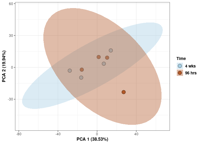
Scree plot and summary statistics hypothalamus
tdata.FPKM.sample.info <- readRDS(here("Data","20190406_RNAseq_B6_4wk_2DG_counts_phenotypes.RData"))
tdata.FPKM.sample.info.hypothalamus <- rownames_to_column(tdata.FPKM.sample.info) %>% filter(Tissue=="Hypothanamus" & Treatment=="None") %>% column_to_rownames('rowname')
tdata.FPKM <- readRDS(here("Data","20190406_RNAseq_B6_4wk_2DG_counts_numeric.RData"))
log.tdata.FPKM <- log(tdata.FPKM + 1)
log.tdata.FPKM <- as.data.frame(log.tdata.FPKM)
rows <- rownames(tdata.FPKM.sample.info.hypothalamus)
log.tdata.FPKM.hypothalamus <- rownames_to_column(log.tdata.FPKM)
log.tdata.FPKM.hypothalamus <- log.tdata.FPKM.hypothalamus %>% filter(rowname %in% rows) %>% column_to_rownames('rowname')
pca <- prcomp(log.tdata.FPKM.hypothalamus, center = T)
screeplot(pca,type = "lines")
summary(pca)## Importance of components:
## PC1 PC2 PC3 PC4 PC5 PC6 PC7
## Standard deviation 18.6969 12.4851 11.2748 10.3039 9.09885 7.71606 7.10209
## Proportion of Variance 0.3753 0.1673 0.1365 0.1140 0.08888 0.06392 0.05415
## Cumulative Proportion 0.3753 0.5426 0.6791 0.7931 0.88194 0.94585 1.00000
## PC8
## Standard deviation 1.777e-14
## Proportion of Variance 0.000e+00
## Cumulative Proportion 1.000e+00Time hypothalamus
Time_color <- as.factor(tdata.FPKM.sample.info.hypothalamus$Time)
Time_color <- as.data.frame(Time_color)
col_time <- colorRampPalette(brewer.pal(n = 12, name = "Paired"))(2)[Time_color$Time_color]
pca_time <- cbind(Time_color,pca$x[,1],pca$x[,2])
pca_time <- as.data.frame(pca_time)
p <- ggplot(pca_time,aes(pca$x[,1], pca$x[,2]))
p <- p + geom_point(aes(fill = as.factor(pca_time$Time_color)), shape=21, size=4) + theme_bw()
p <- p + theme(legend.title = element_text(size=10,face="bold")) +
theme(legend.text = element_text(size=10, face="bold"))
p <- p + xlab("PCA 1 (38.53%)") + ylab("PCA 2 (19.94%)") + theme(axis.title = element_text(face="bold"))
p <- p + stat_ellipse(aes(pca$x[,1], pca$x[,2], group = Time_color, fill = as.factor(pca_time$Time_color)), geom="polygon",level=0.95,alpha=0.4) +
scale_fill_manual(values=c("#A6CEE3", "#B15928"),name="Time",
breaks=c("4 wks", "96 hrs"),
labels=c("4 wks", "96 hrs")) +
scale_linetype_manual(values=c(1,2))
print(p)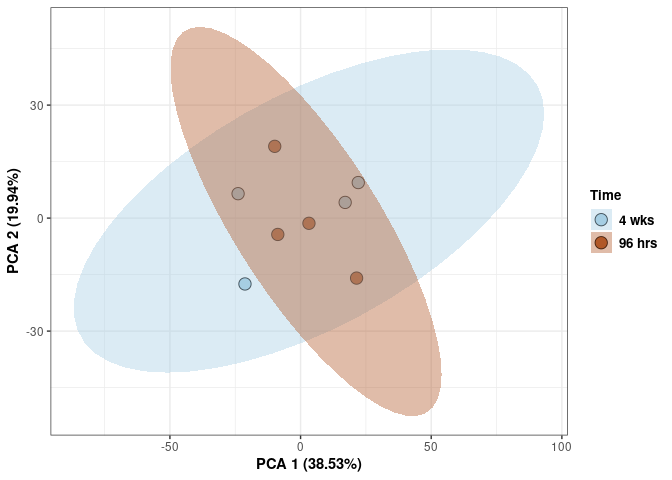
Scree plot and summary statistics hippocampus
tdata.FPKM.sample.info <- readRDS(here("Data","20190406_RNAseq_B6_4wk_2DG_counts_phenotypes.RData"))
tdata.FPKM.sample.info.hippocampus <- rownames_to_column(tdata.FPKM.sample.info) %>% filter(Tissue=="Hippocampus" & Treatment=="None") %>% column_to_rownames('rowname')
tdata.FPKM <- readRDS(here("Data","20190406_RNAseq_B6_4wk_2DG_counts_numeric.RData"))
log.tdata.FPKM <- log(tdata.FPKM + 1)
log.tdata.FPKM <- as.data.frame(log.tdata.FPKM)
rows <- rownames(tdata.FPKM.sample.info.hippocampus)
log.tdata.FPKM.hippocampus <- rownames_to_column(log.tdata.FPKM)
log.tdata.FPKM.hippocampus <- log.tdata.FPKM.hippocampus %>% filter(rowname %in% rows) %>% column_to_rownames('rowname')
pca <- prcomp(log.tdata.FPKM.hippocampus, center = T)
screeplot(pca,type = "lines")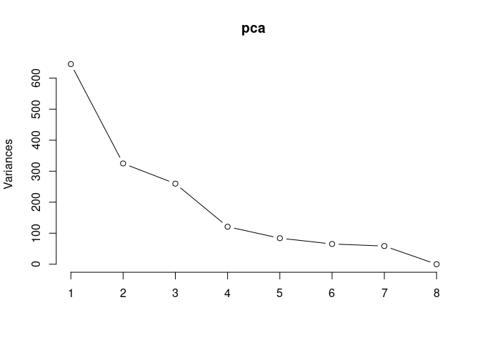
summary(pca)## Importance of components:
## PC1 PC2 PC3 PC4 PC5 PC6 PC7
## Standard deviation 25.404 18.0255 16.1190 10.99610 9.15985 8.07954 7.65717
## Proportion of Variance 0.414 0.2084 0.1667 0.07757 0.05382 0.04188 0.03761
## Cumulative Proportion 0.414 0.6224 0.7891 0.86668 0.92051 0.96239 1.00000
## PC8
## Standard deviation 1.746e-14
## Proportion of Variance 0.000e+00
## Cumulative Proportion 1.000e+00Time hippocampus
Time_color <- as.factor(tdata.FPKM.sample.info.hippocampus$Time)
Time_color <- as.data.frame(Time_color)
col_time <- colorRampPalette(brewer.pal(n = 12, name = "Paired"))(2)[Time_color$Time_color]
pca_time <- cbind(Time_color,pca$x[,1],pca$x[,2])
pca_time <- as.data.frame(pca_time)
p <- ggplot(pca_time,aes(pca$x[,1], pca$x[,2]))
p <- p + geom_point(aes(fill = as.factor(pca_time$Time_color)), shape=21, size=4) + theme_bw()
p <- p + theme(legend.title = element_text(size=10,face="bold")) +
theme(legend.text = element_text(size=10, face="bold"))
p <- p + xlab("PCA 1 (38.53%)") + ylab("PCA 2 (19.94%)") + theme(axis.title = element_text(face="bold"))
p <- p + stat_ellipse(aes(pca$x[,1], pca$x[,2], group = Time_color, fill = as.factor(pca_time$Time_color)), geom="polygon",level=0.95,alpha=0.4) +
scale_fill_manual(values=c("#A6CEE3", "#B15928"),name="Time",
breaks=c("4 wks", "96 hrs"),
labels=c("4 wks", "96 hrs")) +
scale_linetype_manual(values=c(1,2))
print(p)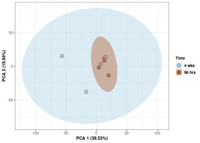
Scree plot and summary statistics liver
tdata.FPKM.sample.info <- readRDS(here("Data","20190406_RNAseq_B6_4wk_2DG_counts_phenotypes.RData"))
tdata.FPKM.sample.info.liver <- rownames_to_column(tdata.FPKM.sample.info) %>% filter(Tissue=="Liver" & Treatment=="None") %>% column_to_rownames('rowname')
tdata.FPKM <- readRDS(here("Data","20190406_RNAseq_B6_4wk_2DG_counts_numeric.RData"))
log.tdata.FPKM <- log(tdata.FPKM + 1)
log.tdata.FPKM <- as.data.frame(log.tdata.FPKM)
rows <- rownames(tdata.FPKM.sample.info.liver)
log.tdata.FPKM.liver <- rownames_to_column(log.tdata.FPKM)
log.tdata.FPKM.liver <- log.tdata.FPKM.liver %>% filter(rowname %in% rows) %>% column_to_rownames('rowname')
pca <- prcomp(log.tdata.FPKM.liver, center = T)
screeplot(pca,type = "lines")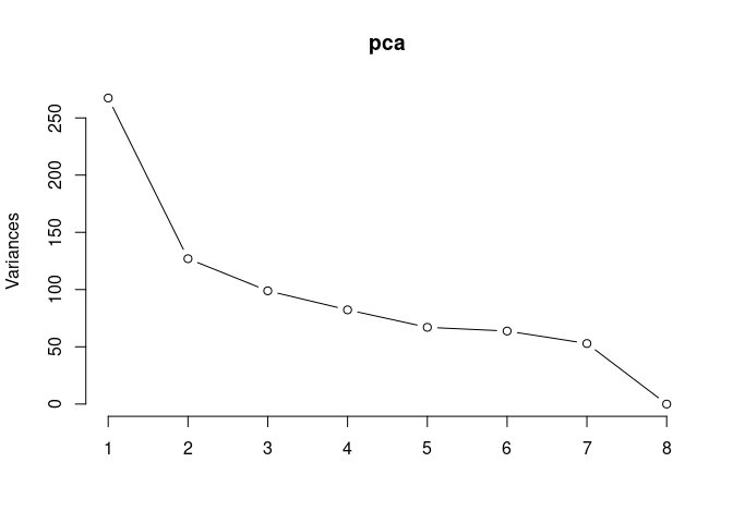
summary(pca)## Importance of components:
## PC1 PC2 PC3 PC4 PC5 PC6 PC7
## Standard deviation 16.3514 11.2690 9.9462 9.0721 8.18875 7.98679 7.27334
## Proportion of Variance 0.3521 0.1672 0.1303 0.1084 0.08831 0.08401 0.06967
## Cumulative Proportion 0.3521 0.5193 0.6496 0.7580 0.84633 0.93033 1.00000
## PC8
## Standard deviation 1.416e-14
## Proportion of Variance 0.000e+00
## Cumulative Proportion 1.000e+00Time liver
Time_color <- as.factor(tdata.FPKM.sample.info.liver$Time)
Time_color <- as.data.frame(Time_color)
col_time <- colorRampPalette(brewer.pal(n = 12, name = "Paired"))(2)[Time_color$Time_color]
pca_time <- cbind(Time_color,pca$x[,1],pca$x[,2])
pca_time <- as.data.frame(pca_time)
p <- ggplot(pca_time,aes(pca$x[,1], pca$x[,2]))
p <- p + geom_point(aes(fill = as.factor(pca_time$Time_color)), shape=21, size=4) + theme_bw()
p <- p + theme(legend.title = element_text(size=10,face="bold")) +
theme(legend.text = element_text(size=10, face="bold"))
p <- p + xlab("PCA 1 (38.53%)") + ylab("PCA 2 (19.94%)") + theme(axis.title = element_text(face="bold"))
p <- p + stat_ellipse(aes(pca$x[,1], pca$x[,2], group = Time_color, fill = as.factor(pca_time$Time_color)), geom="polygon",level=0.95,alpha=0.4) +
scale_fill_manual(values=c("#A6CEE3", "#B15928"),name="Time",
breaks=c("4 wks", "96 hrs"),
labels=c("4 wks", "96 hrs")) +
scale_linetype_manual(values=c(1,2))
print(p)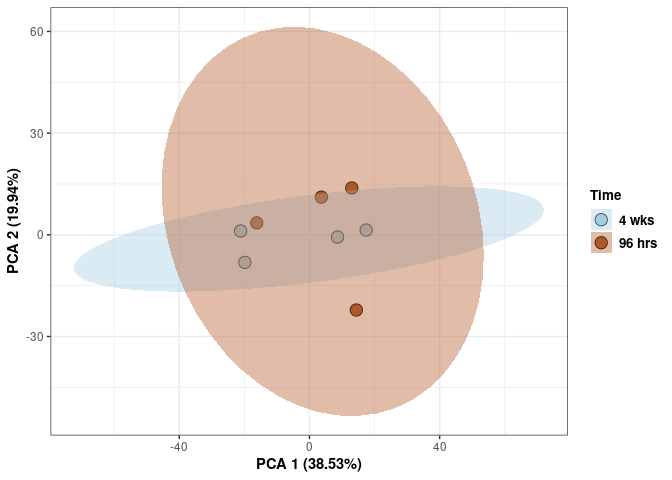
Scree plot and summary statistics heart
tdata.FPKM.sample.info <- readRDS(here("Data","20190406_RNAseq_B6_4wk_2DG_counts_phenotypes.RData"))
tdata.FPKM.sample.info.heart <- rownames_to_column(tdata.FPKM.sample.info) %>% filter(Tissue=="Heart" & Treatment=="None") %>% column_to_rownames('rowname')
tdata.FPKM <- readRDS(here("Data","20190406_RNAseq_B6_4wk_2DG_counts_numeric.RData"))
log.tdata.FPKM <- log(tdata.FPKM + 1)
log.tdata.FPKM <- as.data.frame(log.tdata.FPKM)
rows <- rownames(tdata.FPKM.sample.info.heart)
log.tdata.FPKM.heart <- rownames_to_column(log.tdata.FPKM)
log.tdata.FPKM.heart <- log.tdata.FPKM.heart %>% filter(rowname %in% rows) %>% column_to_rownames('rowname')
pca <- prcomp(log.tdata.FPKM.heart, center = T)
screeplot(pca,type = "lines")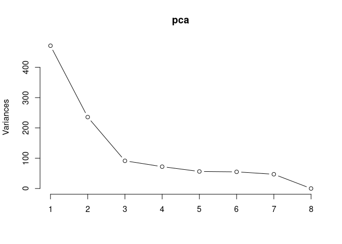
summary(pca)## Importance of components:
## PC1 PC2 PC3 PC4 PC5 PC6 PC7
## Standard deviation 21.7064 15.3509 9.55968 8.48976 7.49644 7.41381 6.86074
## Proportion of Variance 0.4581 0.2291 0.08885 0.07008 0.05464 0.05344 0.04576
## Cumulative Proportion 0.4581 0.6872 0.77608 0.84616 0.90079 0.95424 1.00000
## PC8
## Standard deviation 1.366e-14
## Proportion of Variance 0.000e+00
## Cumulative Proportion 1.000e+00Time heart
Time_color <- as.factor(tdata.FPKM.sample.info.heart$Time)
Time_color <- as.data.frame(Time_color)
col_time <- colorRampPalette(brewer.pal(n = 12, name = "Paired"))(2)[Time_color$Time_color]
pca_time <- cbind(Time_color,pca$x[,1],pca$x[,2])
pca_time <- as.data.frame(pca_time)
p <- ggplot(pca_time,aes(pca$x[,1], pca$x[,2]))
p <- p + geom_point(aes(fill = as.factor(pca_time$Time_color)), shape=21, size=4) + theme_bw()
p <- p + theme(legend.title = element_text(size=10,face="bold")) +
theme(legend.text = element_text(size=10, face="bold"))
p <- p + xlab("PCA 1 (38.53%)") + ylab("PCA 2 (19.94%)") + theme(axis.title = element_text(face="bold"))
p <- p + stat_ellipse(aes(pca$x[,1], pca$x[,2], group = Time_color, fill = as.factor(pca_time$Time_color)), geom="polygon",level=0.95,alpha=0.4) +
scale_fill_manual(values=c("#A6CEE3", "#B15928"),name="Time",
breaks=c("4 wks", "96 hrs"),
labels=c("4 wks", "96 hrs")) +
scale_linetype_manual(values=c(1,2))
print(p)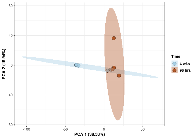
Scree plot and summary statistics small intestine
tdata.FPKM.sample.info <- readRDS(here("Data","20190406_RNAseq_B6_4wk_2DG_counts_phenotypes.RData"))
tdata.FPKM.sample.info.small.intestine <- rownames_to_column(tdata.FPKM.sample.info) %>% filter(Tissue=="Small Intestine" & Treatment=="None") %>% column_to_rownames('rowname')
tdata.FPKM <- readRDS(here("Data","20190406_RNAseq_B6_4wk_2DG_counts_numeric.RData"))
log.tdata.FPKM <- log(tdata.FPKM + 1)
log.tdata.FPKM <- as.data.frame(log.tdata.FPKM)
rows <- rownames(tdata.FPKM.sample.info.small.intestine)
log.tdata.FPKM.small.intestine <- rownames_to_column(log.tdata.FPKM)
log.tdata.FPKM.small.intestine <- log.tdata.FPKM.small.intestine %>% filter(rowname %in% rows) %>% column_to_rownames('rowname')
pca <- prcomp(log.tdata.FPKM.small.intestine, center = T)
screeplot(pca,type = "lines")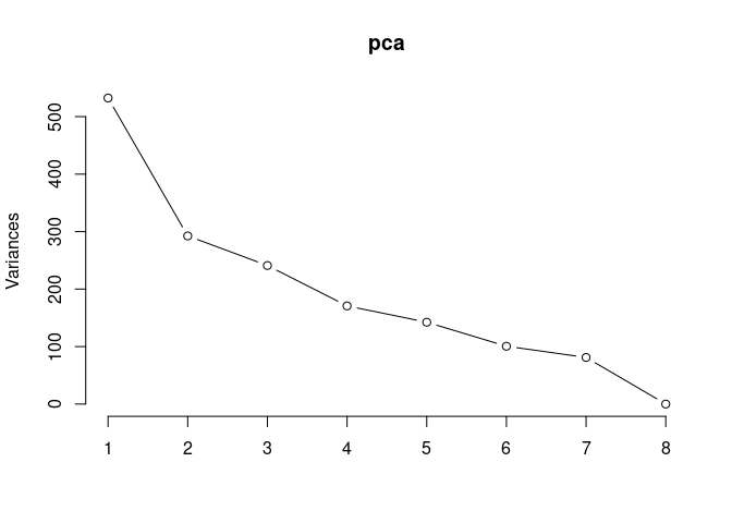
summary(pca)## Importance of components:
## PC1 PC2 PC3 PC4 PC5 PC6
## Standard deviation 23.0733 17.1002 15.5241 13.0670 11.93186 10.02898
## Proportion of Variance 0.3412 0.1874 0.1544 0.1094 0.09123 0.06445
## Cumulative Proportion 0.3412 0.5285 0.6830 0.7924 0.88360 0.94805
## PC7 PC8
## Standard deviation 9.00357 1.729e-14
## Proportion of Variance 0.05195 0.000e+00
## Cumulative Proportion 1.00000 1.000e+00Time small intestine
Time_color <- as.factor(tdata.FPKM.sample.info.small.intestine$Time)
Time_color <- as.data.frame(Time_color)
col_time <- colorRampPalette(brewer.pal(n = 12, name = "Paired"))(2)[Time_color$Time_color]
pca_time <- cbind(Time_color,pca$x[,1],pca$x[,2])
pca_time <- as.data.frame(pca_time)
p <- ggplot(pca_time,aes(pca$x[,1], pca$x[,2]))
p <- p + geom_point(aes(fill = as.factor(pca_time$Time_color)), shape=21, size=4) + theme_bw()
p <- p + theme(legend.title = element_text(size=10,face="bold")) +
theme(legend.text = element_text(size=10, face="bold"))
p <- p + xlab("PCA 1 (38.53%)") + ylab("PCA 2 (19.94%)") + theme(axis.title = element_text(face="bold"))
p <- p + stat_ellipse(aes(pca$x[,1], pca$x[,2], group = Time_color, fill = as.factor(pca_time$Time_color)), geom="polygon",level=0.95,alpha=0.4) +
scale_fill_manual(values=c("#A6CEE3", "#B15928"),name="Time",
breaks=c("4 wks", "96 hrs"),
labels=c("4 wks", "96 hrs")) +
scale_linetype_manual(values=c(1,2))
print(p)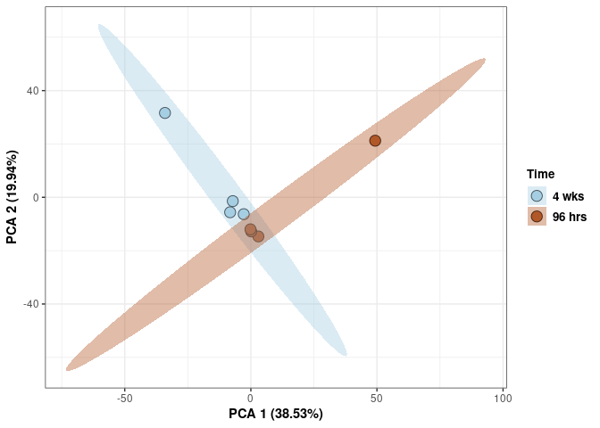
Scree plot and summary statistics skeletal muscle
tdata.FPKM.sample.info <- readRDS(here("Data","20190406_RNAseq_B6_4wk_2DG_counts_phenotypes.RData"))
tdata.FPKM.sample.info.skeletal.muscle <- rownames_to_column(tdata.FPKM.sample.info) %>% filter(Tissue=="Skeletal Muscle" & Treatment=="None") %>% column_to_rownames('rowname')
tdata.FPKM <- readRDS(here("Data","20190406_RNAseq_B6_4wk_2DG_counts_numeric.RData"))
log.tdata.FPKM <- log(tdata.FPKM + 1)
log.tdata.FPKM <- as.data.frame(log.tdata.FPKM)
rows <- rownames(tdata.FPKM.sample.info.skeletal.muscle)
log.tdata.FPKM.skeletal.muscle <- rownames_to_column(log.tdata.FPKM)
log.tdata.FPKM.skeletal.muscle <- log.tdata.FPKM.skeletal.muscle %>% filter(rowname %in% rows) %>% column_to_rownames('rowname')
pca <- prcomp(log.tdata.FPKM.skeletal.muscle, center = T)
screeplot(pca,type = "lines")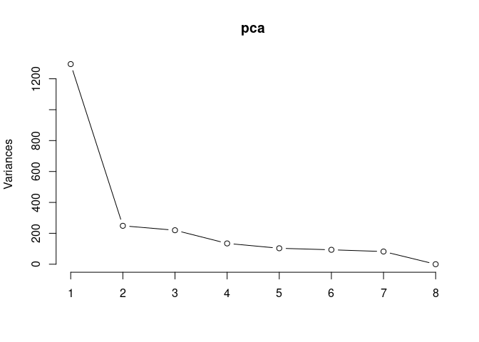
summary(pca)## Importance of components:
## PC1 PC2 PC3 PC4 PC5 PC6
## Standard deviation 35.9869 15.7696 14.8311 11.60231 10.16295 9.66575
## Proportion of Variance 0.5948 0.1142 0.1010 0.06183 0.04744 0.04291
## Cumulative Proportion 0.5948 0.7090 0.8101 0.87189 0.91933 0.96224
## PC7 PC8
## Standard deviation 9.06762 1.35e-14
## Proportion of Variance 0.03776 0.00e+00
## Cumulative Proportion 1.00000 1.00e+00Time skeletal muscle
Time_color <- as.factor(tdata.FPKM.sample.info.skeletal.muscle$Time)
Time_color <- as.data.frame(Time_color)
col_time <- colorRampPalette(brewer.pal(n = 12, name = "Paired"))(2)[Time_color$Time_color]
pca_time <- cbind(Time_color,pca$x[,1],pca$x[,2])
pca_time <- as.data.frame(pca_time)
p <- ggplot(pca_time,aes(pca$x[,1], pca$x[,2]))
p <- p + geom_point(aes(fill = as.factor(pca_time$Time_color)), shape=21, size=4) + theme_bw()
p <- p + theme(legend.title = element_text(size=10,face="bold")) +
theme(legend.text = element_text(size=10, face="bold"))
p <- p + xlab("PCA 1 (38.53%)") + ylab("PCA 2 (19.94%)") + theme(axis.title = element_text(face="bold"))
p <- p + stat_ellipse(aes(pca$x[,1], pca$x[,2], group = Time_color, fill = as.factor(pca_time$Time_color)), geom="polygon",level=0.95,alpha=0.4) +
scale_fill_manual(values=c("#A6CEE3", "#B15928"),name="Time",
breaks=c("4 wks", "96 hrs"),
labels=c("4 wks", "96 hrs")) +
scale_linetype_manual(values=c(1,2))
print(p)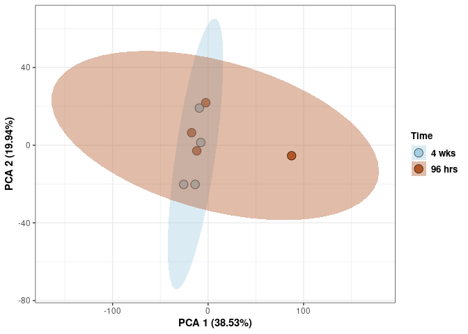
Scree plot and summary statistics prefrontal cortex
tdata.FPKM.sample.info <- readRDS(here("Data","20190406_RNAseq_B6_4wk_2DG_counts_phenotypes.RData"))
tdata.FPKM.sample.info.prefrontal.cortex <- rownames_to_column(tdata.FPKM.sample.info) %>% filter(Tissue=="Pre-frontal Cortex" & Treatment=="None") %>% column_to_rownames('rowname')
tdata.FPKM <- readRDS(here("Data","20190406_RNAseq_B6_4wk_2DG_counts_numeric.RData"))
log.tdata.FPKM <- log(tdata.FPKM + 1)
log.tdata.FPKM <- as.data.frame(log.tdata.FPKM)
rows <- rownames(tdata.FPKM.sample.info.prefrontal.cortex)
log.tdata.FPKM.prefrontal.cortex <- rownames_to_column(log.tdata.FPKM)
log.tdata.FPKM.prefrontal.cortex <- log.tdata.FPKM.prefrontal.cortex %>% filter(rowname %in% rows) %>% column_to_rownames('rowname')
pca <- prcomp(log.tdata.FPKM.prefrontal.cortex, center = T)
screeplot(pca,type = "lines")
summary(pca)## Importance of components:
## PC1 PC2 PC3 PC4 PC5 PC6 PC7
## Standard deviation 20.2225 16.8774 12.8790 9.58862 9.2924 8.47312 7.86336
## Proportion of Variance 0.3491 0.2431 0.1416 0.07848 0.0737 0.06128 0.05278
## Cumulative Proportion 0.3491 0.5922 0.7338 0.81224 0.8859 0.94722 1.00000
## PC8
## Standard deviation 1.728e-14
## Proportion of Variance 0.000e+00
## Cumulative Proportion 1.000e+00Time prefrontal cortex
Time_color <- as.factor(tdata.FPKM.sample.info.prefrontal.cortex$Time)
Time_color <- as.data.frame(Time_color)
col_time <- colorRampPalette(brewer.pal(n = 12, name = "Paired"))(2)[Time_color$Time_color]
pca_time <- cbind(Time_color,pca$x[,1],pca$x[,2])
pca_time <- as.data.frame(pca_time)
p <- ggplot(pca_time,aes(pca$x[,1], pca$x[,2]))
p <- p + geom_point(aes(fill = as.factor(pca_time$Time_color)), shape=21, size=4) + theme_bw()
p <- p + theme(legend.title = element_text(size=10,face="bold")) +
theme(legend.text = element_text(size=10, face="bold"))
p <- p + xlab("PCA 1 (38.53%)") + ylab("PCA 2 (19.94%)") + theme(axis.title = element_text(face="bold"))
p <- p + stat_ellipse(aes(pca$x[,1], pca$x[,2], group = Time_color, fill = as.factor(pca_time$Time_color)), geom="polygon",level=0.95,alpha=0.4) +
scale_fill_manual(values=c("#A6CEE3", "#B15928"),name="Time",
breaks=c("4 wks", "96 hrs"),
labels=c("4 wks", "96 hrs")) +
scale_linetype_manual(values=c(1,2))
print(p)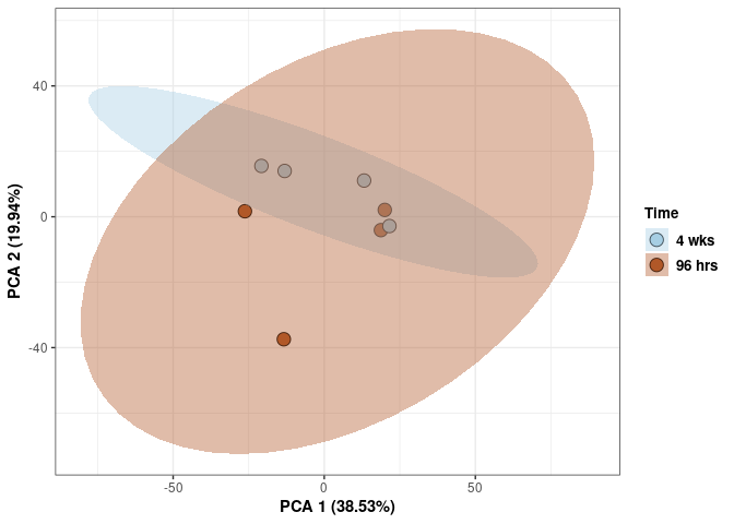
Analysis performed by Ann Wells
The Carter Lab The Jackson Laboratory 2023
ann.wells@jax.org