Module Generation Liver
Ann Wells
April 23, 2023
log.tdata.FPKM.sample.info.subset.liver.WGCNA <- readRDS(here("Data","Liver","log.tdata.FPKM.sample.info.subset.liver.missing.WGCNA.RData"))Set Up Environment
The WGCNA package requires some strict R session environment set up.
options(stringsAsFactors=FALSE)

# Run the following only if running from terminal
# Does NOT work in RStudio
#enableWGCNAThreads()
Choosing Soft-Thresholding Power
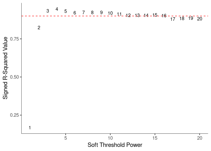
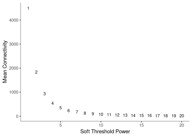
WGCNA uses a smooth softmax function to force a scale-free topology on the gene expression network. I cycled through a set of threshold power values to see which one is the best for the specific topology. As recommended by the authors, I choose the smallest power such that the scale-free topology correlation attempts to hit 0.9.
threshold <- softthreshold(soft)Scale Free Topology
Mean Connectivity
Pick Soft Threshold
knitr::kable(soft$fitIndices)| Power | SFT.R.sq | slope | truncated.R.sq | mean.k. | median.k. | max.k. |
|---|---|---|---|---|---|---|
| 1 | 0.1676528 | -0.7406579 | 0.4121981 | 4499.49707 | 4241.055886 | 6940.8574 |
| 2 | 0.8233717 | -1.2662434 | 0.8360069 | 1837.53642 | 1546.551878 | 4095.0359 |
| 3 | 0.9331752 | -1.3770692 | 0.9232597 | 934.21706 | 679.017891 | 2824.6421 |
| 4 | 0.9467113 | -1.4014966 | 0.9357120 | 544.14677 | 336.917903 | 2135.8386 |
| 5 | 0.9309819 | -1.4086437 | 0.9193551 | 347.60495 | 186.808962 | 1697.4075 |
| 6 | 0.9206839 | -1.4071824 | 0.9114456 | 237.24870 | 108.794320 | 1393.6070 |
| 7 | 0.9242562 | -1.3970730 | 0.9191278 | 170.12157 | 66.829971 | 1170.6657 |
| 8 | 0.9233451 | -1.3917799 | 0.9232094 | 126.71113 | 43.437328 | 1000.2308 |
| 9 | 0.9226327 | -1.3901466 | 0.9287457 | 97.25505 | 29.378261 | 865.9058 |
| 10 | 0.9192027 | -1.3899702 | 0.9304838 | 76.48167 | 20.087376 | 758.5059 |
| 11 | 0.9125883 | -1.3908586 | 0.9318177 | 61.36282 | 13.995328 | 670.4846 |
| 12 | 0.9046831 | -1.3934242 | 0.9313136 | 50.06803 | 10.000650 | 596.9870 |
| 13 | 0.9044865 | -1.3903093 | 0.9370619 | 41.44257 | 7.318231 | 534.8352 |
| 14 | 0.9047933 | -1.3955213 | 0.9434850 | 34.73115 | 5.442770 | 481.7141 |
| 15 | 0.9065988 | -1.3939986 | 0.9491630 | 29.42419 | 4.070167 | 435.8951 |
| 16 | 0.9021656 | -1.4000051 | 0.9494750 | 25.16853 | 3.091694 | 396.0608 |
| 17 | 0.8804805 | -1.4193153 | 0.9365922 | 21.71368 | 2.391115 | 361.1888 |
| 18 | 0.8833739 | -1.4207172 | 0.9413172 | 18.87824 | 1.855614 | 330.4737 |
| 19 | 0.8867793 | -1.4120067 | 0.9503302 | 16.52846 | 1.460437 | 303.2721 |
| 20 | 0.8825087 | -1.4071567 | 0.9529080 | 14.56413 | 1.151573 | 279.0638 |
soft$fitIndices %>%
  download_this(
    output_name = "Soft Threshold Liver",
    output_extension = ".csv",
    button_label = "Download data as csv",
    button_type = "info",
    has_icon = TRUE,
    icon = "fa fa-save"
)Calculate Adjacency Matrix and Topological Overlap Matrix
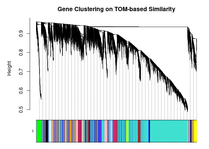
I generated a weighted adjacency matrix for the gene expression profile network using the softmax threshold I determined in the previous step. Then I generate the Topological Overlap Matrix (TOM) for the adjacency matrix. This reduces noise and spurious associations according to the authors.I use the TOM matrix to cluster the profiles of each metabolite based on their similarity. I use dynamic tree cutting to generate modules.
soft.power <- which(soft$fitIndices$SFT.R.sq >= 0.88)[1]
cat("\n", "Power chosen")
##
## Power chosensoft.power## [1] 3cat("\n \n")adj.mtx <- adjacency(log.tdata.FPKM.sample.info.subset.liver.WGCNA, power=soft.power)
TOM = TOMsimilarity(adj.mtx)## ..connectivity..
## ..matrix multiplication (system BLAS)..
## ..normalization..
## ..done.diss.TOM = 1 - TOM
metabolite.clust <- hclust(as.dist(diss.TOM), method="average")
min.module.size <- 15
modules <- cutreeDynamic(dendro=metabolite.clust, distM=diss.TOM, deepSplit=2, pamRespectsDendro=FALSE, minClusterSize=min.module.size)## ..cutHeight not given, setting it to 0.959 ===> 99% of the (truncated) height range in dendro.
## ..done.# Plot modules
cols <- labels2colors(modules)
table(cols)## cols
## bisque4 black blue brown brown4
## 41 375 1289 824 46
## cyan darkgreen darkgrey darkmagenta darkolivegreen
## 189 125 117 87 89
## darkorange darkorange2 darkred darkslateblue darkturquoise
## 104 52 135 41 121
## floralwhite green greenyellow grey60 ivory
## 52 480 255 162 52
## lightcyan lightcyan1 lightgreen lightsteelblue1 lightyellow
## 187 53 159 54 157
## magenta mediumpurple3 midnightblue orange orangered4
## 310 57 187 111 59
## paleturquoise pink plum1 plum2 purple
## 91 338 63 40 287
## red royalblue saddlebrown salmon sienna3
## 465 136 96 194 76
## skyblue skyblue3 steelblue tan thistle2
## 98 67 92 255 35
## turquoise violet white yellow yellowgreen
## 7909 90 100 539 69plotDendroAndColors(
metabolite.clust, cols, xlab="", sub="", main="Gene Clustering on TOM-based Similarity",
dendroLabels=FALSE, hang=0.03, addGuide=TRUE, guideHang=0.05
)
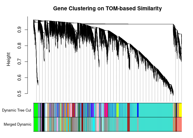
Merging Related Modules
Some modules might be highly correlated. The authors recommend merging modules with a correlation greater than 0.75.
me.list <- moduleEigengenes(log.tdata.FPKM.sample.info.subset.liver.WGCNA, colors=cols)
me <- me.list$eigengenes

# Eigenmetabolite dissimilarity
me.diss <- 1 - cor(me)

h <- hclust(as.dist(me.diss), method="average")

# Merge threshold = 1 - correlation threshold
merge.thresh <- 0.25

plot(h, main="Clustering of Module Eigengene", xlab="", sub="")
abline(h=merge.thresh, col="red")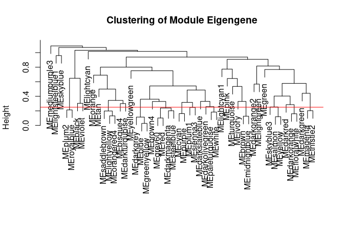
merge <- mergeCloseModules(log.tdata.FPKM.sample.info.subset.liver.WGCNA, cols, cutHeight=merge.thresh, verbose=0)
merged.cols <- merge$colors
merged.mes <- merge$newMEs

  # Check how the merging changed the clustering of the metabolites
plotDendroAndColors(
  metabolite.clust, cbind(cols, merged.cols), c("Dynamic Tree Cut", "Merged Dynamic"), xlab="", sub="",
  main="Gene Clustering on TOM-based Similarity",
  dendroLabels=FALSE, hang=0.03, addGuide=TRUE, guideHang=0.05
  )
Calculating Intramodular Connectivity
This function in WGCNA calculates the total connectivity of a node (metabolite) in the network. The kTotal column specifies this connectivity. The kWithin column specifies the node connectivity within its module. The kOut column specifies the difference between kTotal and kWithin. Generally, the out degree should be lower than the within degree, since the WGCNA procedure groups similar metabolite profiles together.
net.deg <- intramodularConnectivity(adj.mtx, merged.cols)
saveRDS(net.deg,here("Data","Liver","Chang_2DG_BL6_connectivity_liver.RData"))
head(net.deg)
## kTotal kWithin kOut kDiff
## ENSMUSG00000000001 1438.8692 1123.35965 315.5095 807.850150
## ENSMUSG00000000028 435.1013 221.51747 213.5838 7.933677
## ENSMUSG00000000031 883.0249 165.19496 717.8299 -552.634964
## ENSMUSG00000000037 506.8853 23.07137 483.8140 -460.742602
## ENSMUSG00000000049 604.7389 24.80179 579.9371 -555.135345
## ENSMUSG00000000056 579.9107 391.64435 188.2663 203.378039Summary
The dataset generated coexpression modules of the following sizes. The grey submodule represents metabolites that did not fit well into any of the modules.
table(merged.cols)## merged.cols
## bisque4 black brown brown4 cyan
## 41 375 1011 46 615
## darkgreen darkgrey darkolivegreen darkorange darkorange2
## 125 1661 280 156 52
## darkred darkslateblue darkturquoise green grey60
## 135 41 121 480 1463
## ivory lightcyan lightcyan1 lightgreen lightsteelblue1
## 52 187 53 159 54
## mediumpurple3 orange pink plum2 salmon
## 57 111 338 176 733
## skyblue skyblue3 tan turquoise violet
## 98 67 255 7909 90
## yellowgreen
## 69# Module names in descending order of size
module.labels <- names(table(merged.cols))[order(table(merged.cols), decreasing=T)]
# Order eigenmetabolites by module labels
merged.mes <- merged.mes[,paste0("ME", module.labels)]
colnames(merged.mes) <- paste0("log.tdata.FPKM.sample.info.subset.liver.WGCNA_", module.labels)
module.eigens <- merged.mes
# Add log.tdata.FPKM.sample.info.subset.WGCNA tag to labels
module.labels <- paste0("log.tdata.FPKM.sample.info.subset.liver.WGCNA_", module.labels)
# Generate and store metabolite membership
module.membership <- data.frame(
Gene=colnames(log.tdata.FPKM.sample.info.subset.liver.WGCNA),
Module=paste0("log.tdata.FPKM.sample.info.subset.liver.WGCNA_", merged.cols)
)
saveRDS(module.labels, here("Data","Liver","log.tdata.FPKM.sample.info.subset.liver.WGCNA.module.labels.RData"))
saveRDS(module.eigens, here("Data","Liver","log.tdata.FPKM.sample.info.subset.liver.WGCNA.module.eigens.RData"))
saveRDS(module.membership, here("Data","Liver", "log.tdata.FPKM.sample.info.subset.liver.WGCNA.module.membership.RData"))
write.table(module.labels, here("Data","Liver","log.tdata.FPKM.sample.info.subset.liver.WGCNA.module.labels.csv"), row.names=F, col.names=F, sep=",")
write.csv(module.eigens, here("Data","Liver","log.tdata.FPKM.sample.info.subset.liver.WGCNA.module.eigens.csv"))
write.csv(module.membership, here("Data","Liver","log.tdata.FPKM.sample.info.subset.liver.WGCNA.module.membership.csv"), row.names=F)Analysis performed by Ann Wells
The Carter Lab The Jackson Laboratory 2023
ann.wells@jax.org