Module Generation Prefrontal Cortex
Ann Wells
April 23, 2023
log.tdata.FPKM.sample.info.subset.prefrontal.cortex.WGCNA <- readRDS(here("Data","Prefrontal Cortex","log.tdata.FPKM.sample.info.subset.prefrontal.cortex.missing.WGCNA.RData"))Set Up Environment
The WGCNA package requires some strict R session environment set up.
options(stringsAsFactors=FALSE)

# Run the following only if running from terminal
# Does NOT work in RStudio
#enableWGCNAThreads()
Choosing Soft-Thresholding Power
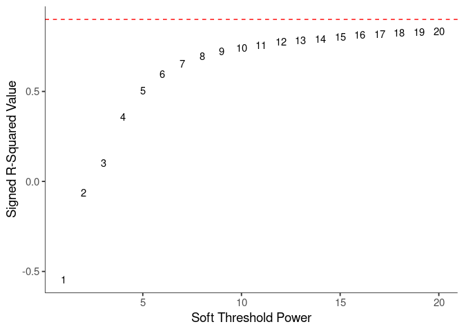
WGCNA uses a smooth softmax function to force a scale-free topology on the gene expression network. I cycled through a set of threshold power values to see which one is the best for the specific topology. As recommended by the authors, I choose the smallest power such that the scale-free topology correlation attempts to hit 0.9.
threshold <- softthreshold(soft)Scale Free Topology
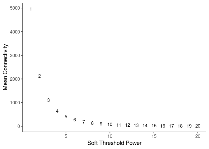
Mean Connectivity
Pick Soft Threshold
knitr::kable(soft$fitIndices)| Power | SFT.R.sq | slope | truncated.R.sq | mean.k. | median.k. | max.k. |
|---|---|---|---|---|---|---|
| 1 | 0.5465425 | 2.9665100 | 0.9429054 | 4970.78415 | 5074.296364 | 6691.3976 |
| 2 | 0.0644743 | 0.3904906 | 0.8376001 | 2127.09094 | 2158.713796 | 3650.2262 |
| 3 | 0.1015397 | -0.4058008 | 0.8091679 | 1102.81854 | 1093.736628 | 2323.5608 |
| 4 | 0.3570354 | -0.8166773 | 0.8460783 | 642.78117 | 614.707278 | 1613.2215 |
| 5 | 0.5050288 | -1.0541463 | 0.8763005 | 405.77152 | 371.137557 | 1184.4329 |
| 6 | 0.5961136 | -1.1934118 | 0.9078318 | 271.49512 | 235.911706 | 904.2017 |
| 7 | 0.6526853 | -1.2865229 | 0.9267020 | 189.89710 | 156.230844 | 710.4712 |
| 8 | 0.6952292 | -1.3571552 | 0.9427953 | 137.55932 | 106.598458 | 571.5220 |
| 9 | 0.7215724 | -1.4204442 | 0.9496898 | 102.51622 | 75.130573 | 468.4787 |
| 10 | 0.7404023 | -1.4658761 | 0.9549286 | 78.21714 | 54.003876 | 389.7865 |
| 11 | 0.7585837 | -1.5094376 | 0.9590279 | 60.87066 | 39.491017 | 328.3912 |
| 12 | 0.7768269 | -1.5329874 | 0.9654022 | 48.17933 | 29.372079 | 280.1128 |
| 13 | 0.7835730 | -1.5609821 | 0.9659901 | 38.69634 | 22.085292 | 241.1996 |
| 14 | 0.7919351 | -1.5802025 | 0.9675566 | 31.48015 | 16.934274 | 209.3814 |
| 15 | 0.8023885 | -1.5947681 | 0.9705433 | 25.90051 | 13.142257 | 183.0666 |
| 16 | 0.8143300 | -1.6015464 | 0.9736404 | 21.52498 | 10.262051 | 161.0839 |
| 17 | 0.8200639 | -1.6099484 | 0.9736915 | 18.05034 | 8.118358 | 142.5558 |
| 18 | 0.8257282 | -1.6175605 | 0.9742033 | 15.25990 | 6.483738 | 126.8143 |
| 19 | 0.8316685 | -1.6221747 | 0.9749324 | 12.99606 | 5.205528 | 113.3502 |
| 20 | 0.8329838 | -1.6294658 | 0.9729368 | 11.14249 | 4.216264 | 101.7764 |
soft$fitIndices %>%
  download_this(
    output_name = "Soft Threshold Prefrontal Cortex",
    output_extension = ".csv",
    button_label = "Download data as csv",
    button_type = "info",
    has_icon = TRUE,
    icon = "fa fa-save"
)Calculate Adjacency Matrix and Topological Overlap Matrix
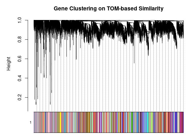
I generated a weighted adjacency matrix for the gene expression profile network using the softmax threshold I determined in the previous step. Then I generate the Topological Overlap Matrix (TOM) for the adjacency matrix. This reduces noise and spurious associations according to the authors.I use the TOM matrix to cluster the profiles of each metabolite based on their similarity. I use dynamic tree cutting to generate modules.
soft.power <- which(soft$fitIndices$SFT.R.sq >= 0.8)[1]
cat("\n", "Power chosen")
##
## Power chosensoft.power## [1] 15cat("\n \n")adj.mtx <- adjacency(log.tdata.FPKM.sample.info.subset.prefrontal.cortex.WGCNA, power=soft.power)
TOM = TOMsimilarity(adj.mtx)## ..connectivity..
## ..matrix multiplication (system BLAS)..
## ..normalization..
## ..done.diss.TOM = 1 - TOM
metabolite.clust <- hclust(as.dist(diss.TOM), method="average")
min.module.size <- 15
modules <- cutreeDynamic(dendro=metabolite.clust, distM=diss.TOM, deepSplit=2, pamRespectsDendro=FALSE, minClusterSize=min.module.size)## ..cutHeight not given, setting it to 0.998 ===> 99% of the (truncated) height range in dendro.
## ..done.# Plot modules
cols <- labels2colors(modules)
table(cols)## cols
## aliceblue antiquewhite antiquewhite1
## 47 40 54
## antiquewhite2 antiquewhite3 antiquewhite4
## 61 32 76
## aquamarine bisque2 bisque3
## 26 23 29
## bisque4 black blanchedalmond
## 83 201 36
## blue blue1 blue2
## 368 44 67
## blue3 blue4 blueviolet
## 49 57 57
## brown brown1 brown2
## 266 49 67
## brown3 brown4 burlywood
## 43 84 35
## burlywood1 burlywood2 chocolate
## 28 23 26
## chocolate1 chocolate2 chocolate3
## 33 40 47
## chocolate4 coral coral1
## 54 62 77
## coral2 coral3 coral4
## 76 61 52
## cornflowerblue cornsilk cornsilk2
## 46 39 32
## cyan cyan1 darkgoldenrod
## 159 26 23
## darkgoldenrod1 darkgoldenrod3 darkgoldenrod4
## 29 36 44
## darkgreen darkgrey darkmagenta
## 124 119 102
## darkolivegreen darkolivegreen1 darkolivegreen2
## 102 49 58
## darkolivegreen4 darkorange darkorange2
## 67 115 84
## darkorchid3 darkorchid4 darkred
## 17 26 128
## darksalmon darkseagreen darkseagreen1
## 33 40 47
## darkseagreen2 darkseagreen3 darkseagreen4
## 54 62 78
## darkslateblue darkturquoise darkviolet
## 83 123 67
## deeppink deeppink1 deeppink2
## 57 49 43
## deepskyblue deepskyblue4 dodgerblue1
## 35 28 23
## dodgerblue2 dodgerblue3 dodgerblue4
## 22 29 36
## firebrick firebrick2 firebrick3
## 44 50 58
## firebrick4 floralwhite goldenrod3
## 68 86 18
## goldenrod4 green green1
## 26 216 33
## green2 green3 green4
## 40 47 54
## greenyellow grey grey60
## 171 681 135
## honeydew honeydew1 hotpink3
## 62 78 23
## hotpink4 indianred indianred1
## 29 36 44
## indianred2 indianred3 indianred4
## 50 58 69
## ivory khaki2 khaki3
## 86 19 26
## khaki4 lavender lavenderblush
## 33 41 47
## lavenderblush1 lavenderblush2 lavenderblush3
## 55 63 79
## lemonchiffon4 lightblue lightblue1
## 23 29 36
## lightblue2 lightblue3 lightblue4
## 44 50 59
## lightcoral lightcyan lightcyan1
## 69 143 89
## lightgoldenrod3 lightgoldenrod4 lightgoldenrodyellow
## 19 26 33
## lightgreen lightpink lightpink1
## 131 41 47
## lightpink2 lightpink3 lightpink4
## 55 64 80
## lightskyblue lightskyblue1 lightskyblue2
## 23 30 36
## lightskyblue3 lightskyblue4 lightslateblue
## 44 50 59
## lightsteelblue lightsteelblue1 lightyellow
## 70 89 131
## lightyellow4 limegreen linen
## 21 27 34
## magenta magenta1 magenta2
## 182 41 47
## magenta3 magenta4 maroon
## 55 64 80
## mediumorchid mediumorchid1 mediumorchid2
## 75 23 30
## mediumorchid3 mediumorchid4 mediumpurple
## 37 44 50
## mediumpurple1 mediumpurple2 mediumpurple3
## 59 70 91
## mediumpurple4 midnightblue mistyrose
## 61 149 52
## mistyrose1 mistyrose2 mistyrose3
## 21 27 34
## mistyrose4 moccasin navajowhite
## 41 47 55
## navajowhite1 navajowhite2 navajowhite3
## 65 80 46
## navajowhite4 oldlace olivedrab4
## 39 31 24
## orange orange1 orange2
## 118 25 30
## orange3 orange4 orangered
## 37 44 51
## orangered1 orangered3 orangered4
## 60 70 92
## palegreen4 paleturquoise paleturquoise1
## 22 104 27
## paleturquoise3 paleturquoise4 palevioletred
## 34 41 48
## palevioletred1 palevioletred2 palevioletred3
## 56 65 81
## peachpuff4 peru pink
## 24 31 193
## pink1 pink2 pink3
## 37 45 51
## pink4 plum plum1
## 60 70 94
## plum2 plum3 plum4
## 82 67 57
## powderblue purple purple2
## 49 172 43
## red red1 red4
## 205 35 28
## rosybrown1 rosybrown2 rosybrown3
## 22 22 27
## rosybrown4 royalblue royalblue2
## 34 128 42
## royalblue3 saddlebrown salmon
## 48 109 161
## salmon1 salmon2 salmon4
## 56 65 81
## seashell3 seashell4 sienna
## 25 31 37
## sienna1 sienna2 sienna3
## 45 52 98
## sienna4 skyblue skyblue1
## 60 111 71
## skyblue2 skyblue3 skyblue4
## 75 94 61
## slateblue slateblue1 slateblue2
## 52 46 38
## slateblue3 slateblue4 steelblue
## 31 25 104
## steelblue3 steelblue4 tan
## 22 28 163
## tan1 tan2 tan3
## 35 43 48
## tan4 thistle thistle1
## 57 66 81
## thistle2 thistle3 thistle4
## 82 66 57
## tomato tomato2 tomato4
## 49 43 35
## turquoise turquoise2 turquoise4
## 526 28 22
## violet violetred4 wheat1
## 102 25 31
## wheat3 white whitesmoke
## 38 111 46
## yellow yellow2 yellow3
## 232 52 60
## yellow4 yellowgreen
## 74 95plotDendroAndColors(
metabolite.clust, cols, xlab="", sub="", main="Gene Clustering on TOM-based Similarity",
dendroLabels=FALSE, hang=0.03, addGuide=TRUE, guideHang=0.05
)
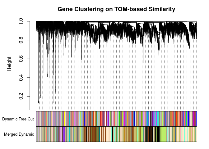
Merging Related Modules
Some modules might be highly correlated. The authors recommend merging modules with a correlation greater than 0.75.
me.list <- moduleEigengenes(log.tdata.FPKM.sample.info.subset.prefrontal.cortex.WGCNA, colors=cols)
me <- me.list$eigengenes

# Eigenmetabolite dissimilarity
me.diss <- 1 - cor(me)

h <- hclust(as.dist(me.diss), method="average")

# Merge threshold = 1 - correlation threshold
merge.thresh <- 0.25

plot(h, main="Clustering of Module Eigengene", xlab="", sub="")
abline(h=merge.thresh, col="red")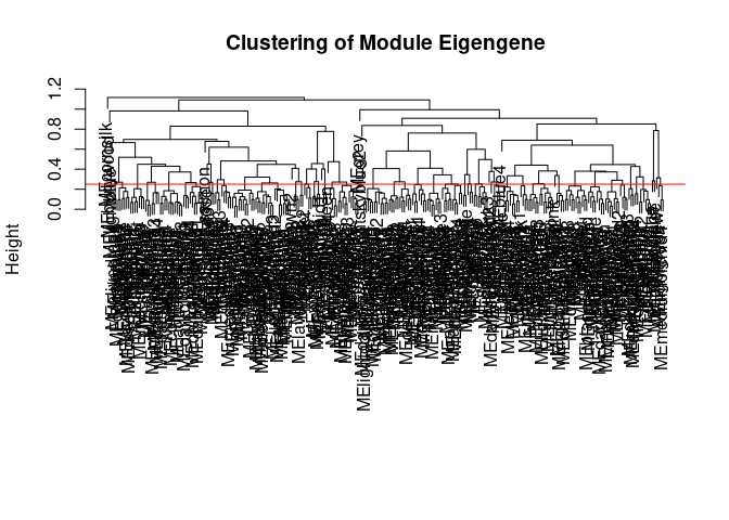
merge <- mergeCloseModules(log.tdata.FPKM.sample.info.subset.prefrontal.cortex.WGCNA, cols, cutHeight=merge.thresh, verbose=0)
merged.cols <- merge$colors
merged.mes <- merge$newMEs

  # Check how the merging changed the clustering of the metabolites
plotDendroAndColors(
  metabolite.clust, cbind(cols, merged.cols), c("Dynamic Tree Cut", "Merged Dynamic"), xlab="", sub="",
  main="Gene Clustering on TOM-based Similarity",
  dendroLabels=FALSE, hang=0.03, addGuide=TRUE, guideHang=0.05
  )
Calculating Intramodular Connectivity
This function in WGCNA calculates the total connectivity of a node (metabolite) in the network. The kTotal column specifies this connectivity. The kWithin column specifies the node connectivity within its module. The kOut column specifies the difference between kTotal and kWithin. Generally, the out degree should be lower than the within degree, since the WGCNA procedure groups similar metabolite profiles together.
net.deg <- intramodularConnectivity(adj.mtx, merged.cols)
saveRDS(net.deg,here("Data","Prefrontal Cortex","Chang_2DG_BL6_connectivity_prefrontal_cortex.RData"))
head(net.deg)
## kTotal kWithin kOut kDiff
## ENSMUSG00000000001 20.6475869 6.56064941 14.0869375 -7.52628806
## ENSMUSG00000000028 0.8270968 0.27883147 0.5482654 -0.26943388
## ENSMUSG00000000031 0.9565852 0.06033695 0.8962482 -0.83591128
## ENSMUSG00000000037 12.0555068 6.80378720 5.2517196 1.55206761
## ENSMUSG00000000049 0.1245447 0.03610669 0.0884380 -0.05233131
## ENSMUSG00000000056 0.5966459 0.26250468 0.3341413 -0.07163659Summary
The dataset generated coexpression modules of the following sizes. The grey submodule represents metabolites that did not fit well into any of the modules.
table(merged.cols)## merged.cols
## antiquewhite aquamarine bisque2 black blanchedalmond
## 201 960 718 2080 2698
## blue4 blueviolet burlywood chocolate2 chocolate4
## 57 372 35 77 2449
## cornsilk cornsilk2 darkolivegreen2 darkolivegreen4 darkseagreen4
## 39 275 1419 681 268
## darkturquoise dodgerblue4 goldenrod3 grey hotpink3
## 360 293 87 681 23
## khaki3 lavenderblush2 lightblue lightgoldenrod3 lightpink1
## 320 110 29 1932 253
## lightskyblue lightskyblue2 limegreen mediumorchid1 mistyrose
## 23 36 27 23 52
## navajowhite3 oldlace pink plum rosybrown2
## 231 31 193 104 22
## salmon
## 161# Module names in descending order of size
module.labels <- names(table(merged.cols))[order(table(merged.cols), decreasing=T)]
# Order eigenmetabolites by module labels
merged.mes <- merged.mes[,paste0("ME", module.labels)]
colnames(merged.mes) <- paste0("log.tdata.FPKM.sample.info.subset.prefrontal.cortex.WGCNA_", module.labels)
module.eigens <- merged.mes
# Add log.tdata.FPKM.sample.info.subset.WGCNA tag to labels
module.labels <- paste0("log.tdata.FPKM.sample.info.subset.prefrontal.cortex.WGCNA_", module.labels)
# Generate and store metabolite membership
module.membership <- data.frame(
Gene=colnames(log.tdata.FPKM.sample.info.subset.prefrontal.cortex.WGCNA),
Module=paste0("log.tdata.FPKM.sample.info.subset.prefrontal.cortex.WGCNA_", merged.cols)
)
saveRDS(module.labels, here("Data","Prefrontal Cortex","log.tdata.FPKM.sample.info.subset.prefrontal.cortex.WGCNA.module.labels.RData"))
saveRDS(module.eigens, here("Data","Prefrontal Cortex","log.tdata.FPKM.sample.info.subset.prefrontal.cortex.WGCNA.module.eigens.RData"))
saveRDS(module.membership, here("Data","Prefrontal Cortex", "log.tdata.FPKM.sample.info.subset.prefrontal.cortex.WGCNA.module.membership.RData"))
write.table(module.labels, here("Data","Prefrontal Cortex","log.tdata.FPKM.sample.info.subset.prefrontal.cortex.WGCNA.module.labels.csv"), row.names=F, col.names=F, sep=",")
write.csv(module.eigens, here("Data","Prefrontal Cortex","log.tdata.FPKM.sample.info.subset.prefrontal.cortex.WGCNA.module.eigens.csv"))
write.csv(module.membership, here("Data","Prefrontal Cortex","log.tdata.FPKM.sample.info.subset.prefrontal.cortex.WGCNA.module.membership.csv"), row.names=F)Analysis performed by Ann Wells
The Carter Lab The Jackson Laboratory 2023
ann.wells@jax.org