Module Generation Spleen
Ann Wells
April 23, 2023
log.tdata.FPKM.sample.info.subset.spleen.WGCNA <- readRDS(here("Data","Spleen","log.tdata.FPKM.sample.info.subset.spleen.missing.WGCNA.RData"))Set Up Environment
The WGCNA package requires some strict R session environment set up.
options(stringsAsFactors=FALSE)

# Run the following only if running from terminal
# Does NOT work in RStudio
#enableWGCNAThreads()
Choosing Soft-Thresholding Power
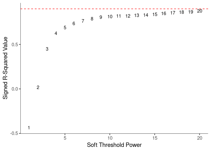
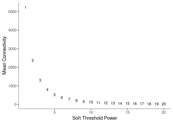
WGCNA uses a smooth softmax function to force a scale-free topology on the gene expression network. I cycled through a set of threshold power values to see which one is the best for the specific topology. As recommended by the authors, I choose the smallest power such that the scale-free topology correlation attempts to hit 0.9.
threshold <- softthreshold(soft)Scale Free Topology
Mean Connectivity
Pick Soft Threshold
knitr::kable(soft$fitIndices)| Power | SFT.R.sq | slope | truncated.R.sq | mean.k. | median.k. | max.k. |
|---|---|---|---|---|---|---|
| 1 | 0.4358270 | 1.7928866 | 0.8458625 | 5240.43008 | 5378.297998 | 7478.0231 |
| 2 | 0.0186294 | -0.1359116 | 0.7059888 | 2372.08988 | 2393.130358 | 4477.4621 |
| 3 | 0.4480157 | -0.6763132 | 0.8107739 | 1299.81369 | 1254.256731 | 3071.2295 |
| 4 | 0.6251143 | -0.9281030 | 0.8646600 | 798.88156 | 722.905146 | 2278.9504 |
| 5 | 0.6912554 | -1.0811030 | 0.8947229 | 530.27905 | 442.943386 | 1781.8218 |
| 6 | 0.7370930 | -1.1697514 | 0.9236377 | 371.97663 | 284.604989 | 1440.8117 |
| 7 | 0.7658612 | -1.2415599 | 0.9442515 | 272.01853 | 190.190056 | 1193.9887 |
| 8 | 0.7904198 | -1.2887483 | 0.9588390 | 205.49509 | 131.058044 | 1008.0899 |
| 9 | 0.8065862 | -1.3325246 | 0.9673574 | 159.35198 | 92.491080 | 865.1887 |
| 10 | 0.8123225 | -1.3706070 | 0.9692731 | 126.25661 | 66.414471 | 752.6934 |
| 11 | 0.8212341 | -1.4014178 | 0.9705356 | 101.85482 | 48.811275 | 661.4014 |
| 12 | 0.8214231 | -1.4337078 | 0.9658009 | 83.44056 | 36.469859 | 586.0772 |
| 13 | 0.8293812 | -1.4519543 | 0.9643297 | 69.26694 | 27.660959 | 523.0560 |
| 14 | 0.8324172 | -1.4758914 | 0.9599573 | 58.16932 | 21.207920 | 470.6965 |
| 15 | 0.8399414 | -1.4822187 | 0.9576177 | 49.34954 | 16.572538 | 426.0696 |
| 16 | 0.8486459 | -1.4844708 | 0.9565516 | 42.24727 | 12.991093 | 387.5125 |
| 17 | 0.8560176 | -1.4815981 | 0.9557554 | 36.46087 | 10.309441 | 353.9346 |
| 18 | 0.8649258 | -1.4802017 | 0.9555574 | 31.69699 | 8.399867 | 324.4873 |
| 19 | 0.8687112 | -1.4793660 | 0.9505068 | 27.73783 | 6.831535 | 298.5007 |
| 20 | 0.8779267 | -1.4690046 | 0.9475410 | 24.41928 | 5.558523 | 275.4398 |
soft$fitIndices %>%
  download_this(
    output_name = "Soft Threshold Spleen",
    output_extension = ".csv",
    button_label = "Download data as csv",
    button_type = "info",
    has_icon = TRUE,
    icon = "fa fa-save"
)Calculate Adjacency Matrix and Topological Overlap Matrix
I generated a weighted adjacency matrix for the gene expression profile network using the softmax threshold I determined in the previous step. Then I generate the Topological Overlap Matrix (TOM) for the adjacency matrix. This reduces noise and spurious associations according to the authors. I use the TOM matrix to cluster the profiles of each metabolite based on their similarity. I use dynamic tree cutting to generate modules.
soft.power <- which(soft$fitIndices$SFT.R.sq >= 0.87)[1]
cat("\n", "Power chosen")
##
## Power chosensoft.power## [1] 20cat("\n \n")adj.mtx <- adjacency(log.tdata.FPKM.sample.info.subset.spleen.WGCNA, power=soft.power)
TOM = TOMsimilarity(adj.mtx)## ..connectivity..
## ..matrix multiplication (system BLAS)..
## ..normalization..
## ..done.diss.TOM = 1 - TOM
metabolite.clust <- hclust(as.dist(diss.TOM), method="average")
min.module.size <- 15
modules <- cutreeDynamic(dendro=metabolite.clust, distM=diss.TOM, deepSplit=2, pamRespectsDendro=FALSE, minClusterSize=min.module.size)## ..cutHeight not given, setting it to 0.998 ===> 99% of the (truncated) height range in dendro.
## ..done.# Plot modules
cols <- labels2colors(modules)
table(cols)## cols
## aliceblue antiquewhite1 antiquewhite2 antiquewhite4 bisque4
## 36 47 63 81 92
## black blue blue2 blue3 blue4
## 243 593 73 42 54
## blueviolet brown brown1 brown2 brown4
## 54 420 42 73 93
## chocolate3 chocolate4 coral coral1 coral2
## 36 48 63 81 81
## coral3 coral4 cornflowerblue cyan darkgreen
## 63 46 34 180 124
## darkgrey darkmagenta darkolivegreen darkolivegreen1 darkolivegreen2
## 120 106 111 42 57
## darkolivegreen4 darkorange darkorange2 darkred darkseagreen1
## 74 114 94 129 37
## darkseagreen2 darkseagreen3 darkseagreen4 darkslateblue darkturquoise
## 48 65 83 92 124
## darkviolet deeppink deeppink1 firebrick firebrick2
## 73 54 42 20 42
## firebrick3 firebrick4 floralwhite green green3
## 57 75 96 291 38
## green4 greenyellow grey grey60 honeydew
## 48 204 2569 146 66
## honeydew1 indianred1 indianred2 indianred3 indianred4
## 84 23 43 58 75
## ivory lavenderblush lavenderblush1 lavenderblush2 lavenderblush3
## 96 38 49 67 84
## lightblue2 lightblue3 lightblue4 lightcoral lightcyan
## 23 44 58 76 146
## lightcyan1 lightgreen lightpink1 lightpink2 lightpink3
## 97 141 38 50 67
## lightpink4 lightskyblue3 lightskyblue4 lightslateblue lightsteelblue
## 85 29 44 58 76
## lightsteelblue1 lightyellow magenta magenta2 magenta3
## 98 139 225 38 50
## magenta4 maroon mediumorchid mediumorchid4 mediumpurple
## 68 86 80 29 44
## mediumpurple1 mediumpurple2 mediumpurple3 mediumpurple4 midnightblue
## 58 77 98 60 152
## mistyrose moccasin navajowhite navajowhite1 navajowhite2
## 46 39 50 68 86
## navajowhite3 orange orange4 orangered orangered1
## 33 115 30 45 60
## orangered3 orangered4 paleturquoise palevioletred palevioletred1
## 77 98 111 39 51
## palevioletred2 palevioletred3 pink pink2 pink3
## 69 87 226 30 45
## pink4 plum plum1 plum2 plum3
## 60 77 99 92 72
## plum4 powderblue purple red royalblue
## 53 42 209 273 132
## royalblue3 saddlebrown salmon salmon1 salmon2
## 39 112 183 52 69
## salmon4 sienna1 sienna2 sienna3 sienna4
## 87 31 45 103 60
## skyblue skyblue1 skyblue2 skyblue3 skyblue4
## 113 78 80 100 60
## slateblue slateblue1 steelblue tan tan3
## 46 33 112 196 40
## tan4 thistle thistle1 thistle2 thistle3
## 52 70 88 90 71
## thistle4 tomato turquoise violet white
## 53 41 968 111 113
## whitesmoke yellow yellow2 yellow3 yellow4
## 32 331 46 60 79
## yellowgreen
## 101plotDendroAndColors(
metabolite.clust, cols, xlab="", sub="", main="Gene Clustering on TOM-based Similarity",
dendroLabels=FALSE, hang=0.03, addGuide=TRUE, guideHang=0.05
)
Merging Related Modules
Some modules might be highly correlated. The authors recommend merging modules with a correlation greater than 0.75.
me.list <- moduleEigengenes(log.tdata.FPKM.sample.info.subset.spleen.WGCNA, colors=cols)
me <- me.list$eigengenes

# Eigenmetabolite dissimilarity
me.diss <- 1 - cor(me)

h <- hclust(as.dist(me.diss), method="average")

# Merge threshold = 1 - correlation threshold
merge.thresh <- 0.25

plot(h, main="Clustering of Module Eigengene", xlab="", sub="")
abline(h=merge.thresh, col="red")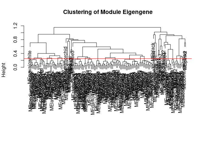
merge <- mergeCloseModules(log.tdata.FPKM.sample.info.subset.spleen.WGCNA, cols, cutHeight=merge.thresh, verbose=0)
merged.cols <- merge$colors
merged.mes <- merge$newMEs
# Check how the merging changed the clustering of the metabolites
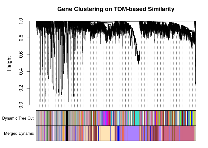
plotDendroAndColors(
metabolite.clust, cbind(cols, merged.cols), c("Dynamic Tree Cut", "Merged Dynamic"), xlab="", sub="",
main="Gene Clustering on TOM-based Similarity",
dendroLabels=FALSE, hang=0.03, addGuide=TRUE, guideHang=0.05
)
Calculating Intramodular Connectivity
This function in WGCNA calculates the total connectivity of a node (metabolite) in the network. The kTotal column specifies this connectivity. The kWithin column specifies the node connectivity within its module. The kOut column specifies the difference between kTotal and kWithin. Generally, the out degree should be lower than the within degree, since the WGCNA procedure groups similar metabolite profiles together.
net.deg <- intramodularConnectivity(adj.mtx, merged.cols)
saveRDS(net.deg,here("Data","Spleen","Chang_2DG_BL6_connectivity_spleen.RData"))
head(net.deg)
## kTotal kWithin kOut kDiff
## ENSMUSG00000000001 92.6485840 88.8976529 3.75093110 85.1467218
## ENSMUSG00000000028 168.8769283 167.5354835 1.34144480 166.1940387
## ENSMUSG00000000031 0.8393023 0.6023274 0.23697496 0.3653524
## ENSMUSG00000000037 1.4076383 0.8654836 0.54215474 0.3233288
## ENSMUSG00000000049 5.2845111 5.2522912 0.03221985 5.2200714
## ENSMUSG00000000056 34.2856976 33.6477921 0.63790551 33.0098866Summary
The dataset generated coexpression modules of the following sizes. The grey submodule represents metabolites that did not fit well into any of the modules.
table(merged.cols)## merged.cols
## black blue2 blue3 brown4 coral2
## 243 289 380 153 571
## cornflowerblue darkgreen darkseagreen3 darkseagreen4 grey
## 34 124 65 83 2569
## indianred1 indianred2 indianred4 lightblue2 lightskyblue4
## 23 43 1466 23 44
## mediumorchid mediumpurple mediumpurple1 moccasin navajowhite
## 80 44 2240 2859 50
## orange orangered4 palevioletred3 pink2 plum
## 194 201 4073 30 77
## royalblue3 sienna2 slateblue1 tan4 thistle1
## 39 45 798 200 178
## thistle3
## 71# Module names in descending order of size
module.labels <- names(table(merged.cols))[order(table(merged.cols), decreasing=T)]
# Order eigenmetabolites by module labels
merged.mes <- merged.mes[,paste0("ME", module.labels)]
colnames(merged.mes) <- paste0("log.tdata.FPKM.sample.info.subset.spleen.WGCNA_", module.labels)
module.eigens <- merged.mes
# Add log.tdata.FPKM.sample.info.subset.WGCNA tag to labels
module.labels <- paste0("log.tdata.FPKM.sample.info.subset.spleen.WGCNA_", module.labels)
# Generate and store metabolite membership
module.membership <- data.frame(
Gene=colnames(log.tdata.FPKM.sample.info.subset.spleen.WGCNA),
Module=paste0("log.tdata.FPKM.sample.info.subset.spleen.WGCNA_", merged.cols)
)
saveRDS(module.labels, here("Data","Spleen","log.tdata.FPKM.sample.info.subset.spleen.WGCNA.module.labels.RData"))
saveRDS(module.eigens, here("Data","Spleen","log.tdata.FPKM.sample.info.subset.spleen.WGCNA.module.eigens.RData"))
saveRDS(module.membership, here("Data","Spleen", "log.tdata.FPKM.sample.info.subset.spleen.WGCNA.module.membership.RData"))
write.table(module.labels, here("Data","Spleen","log.tdata.FPKM.sample.info.subset.spleen.WGCNA.module.labels.csv"), row.names=F, col.names=F, sep=",")
write.csv(module.eigens, here("Data","Spleen","log.tdata.FPKM.sample.info.subset.spleen.WGCNA.module.eigens.csv"))
write.csv(module.membership, here("Data","Spleen","log.tdata.FPKM.sample.info.subset.spleen.WGCNA.module.membership.csv"), row.names=F)Analysis performed by Ann Wells
The Carter Lab The Jackson Laboratory 2023
ann.wells@jax.org