Frequency of Pathways by Module-Trait Relationship Skeletal Muscle
Ann Wells
April 23, 2023
Introduction and Data files
This dataset contains nine tissues (heart, hippocampus, hypothalamus, kidney, liver, prefrontal cortex, skeletal muscle, small intestine, and spleen) from C57BL/6J mice that were fed 2-deoxyglucose (6g/L) through their drinking water for 96hrs or 4wks. 96hr mice were given their 2DG treatment 2 weeks after the other cohort started the 4 week treatment. The organs from the mice were harvested and processed for metabolomics and transcriptomics. The data in this document pertains to the transcriptomics data only. The counts that were used were FPKM normalized before being log transformed. It was determined that sample A113 had low RNAseq quality and through further analyses with PCA, MA plots, and clustering was an outlier and will be removed for the rest of the analyses performed. This document will determine the contribution of each main effect or their combination to each module identified, as well as the relationship of each gene within the module and its significance.
needed.packages <- c("tidyverse", "here", "functional", "gplots", "dplyr", "GeneOverlap", "R.utils", "reshape2","magrittr","data.table", "RColorBrewer","preprocessCore", "ARTool","emmeans", "phia", "gProfileR", "WGCNA","plotly", "pheatmap","downloadthis")
for(i in 1:length(needed.packages)){library(needed.packages[i], character.only = TRUE)}

source(here("source_files","WGCNA_source.R"))
tdata.FPKM.sample.info <- readRDS(here("Data","20190406_RNAseq_B6_4wk_2DG_counts_phenotypes.RData"))
tdata.FPKM <- readRDS(here("Data","20190406_RNAseq_B6_4wk_2DG_counts_numeric.RData"))
log.tdata.FPKM <- log(tdata.FPKM + 1)
log.tdata.FPKM <- as.data.frame(log.tdata.FPKM)
log.tdata.FPKM.sample.info <- cbind(log.tdata.FPKM, tdata.FPKM.sample.info[,27238:27240])
log.tdata.FPKM.sample.info <- log.tdata.FPKM.sample.info %>% rownames_to_column() %>% filter(rowname != "A113") %>% column_to_rownames()
log.tdata.FPKM.subset <- log.tdata.FPKM[,colMeans(log.tdata.FPKM != 0) > 0.5]
log.tdata.FPKM.subset <- log.tdata.FPKM.subset %>% rownames_to_column() %>% filter(rowname != "A113") %>% column_to_rownames()
log.tdata.FPKM.sample.info.subset.skeletal.muscle <- log.tdata.FPKM.sample.info %>% rownames_to_column() %>% filter(Tissue == "Skeletal Muscle") %>% column_to_rownames()
log.tdata.FPKM.subset <- subset(log.tdata.FPKM.sample.info.subset.skeletal.muscle, select = -c(Time,Treatment,Tissue))
WGCNA.pathway <-readRDS(here("Data","Skeletal Muscle","Chang_B6_96hr_4wk_gprofiler_pathway_annotation_list_skeletal_muscle_WGCNA.RData"))
Matched<-readRDS(here("Data","Skeletal Muscle","Annotated_genes_in_skeletal_muscle_WGCNA_Chang_B6_96hr_4wk.RData"))module.names <- Matched$X..Module.
name <- str_split(module.names,"_")
samples <-c()
for(i in 1:length(name)){
samples[[i]] <- name[[i]][2]
}
name <- str_split(samples,"\"")
name <- unlist(name)
Treatment <- unclass(as.factor(log.tdata.FPKM.sample.info.subset.skeletal.muscle[,27238]))
Time <- unclass(as.factor(log.tdata.FPKM.sample.info.subset.skeletal.muscle[,27237]))
Treat.Time <- paste0(Treatment, Time)
phenotype <- data.frame(cbind(Treatment, Time, Treat.Time))
nSamples <- nrow(log.tdata.FPKM.sample.info.subset.skeletal.muscle)
MEs0 <- read.csv(here("Data","Skeletal Muscle","log.tdata.FPKM.sample.info.subset.skeletal.muscle.WGCNA.module.eigens.csv"),header = T, row.names = 1)
name <- str_split(names(MEs0),"_")
samples <-c()
for(i in 1:length(name)){
samples[[i]] <- name[[i]][2]
}
name <- str_split(samples,"\"")
name <- unlist(name)
colnames(MEs0) <-name
MEs <- orderMEs(MEs0)
moduleTraitCor <- cor(MEs, phenotype, use = "p");
moduleTraitPvalue <- corPvalueStudent(moduleTraitCor, nSamples) time.pathways <- list()
treat.pathways <- list()
time.treat.pathways <- list()
for(i in 1:nrow(moduleTraitPvalue)){
if(moduleTraitPvalue[i,2] < 0.05){
time.pathways[[i]] <- WGCNA.pathway[[i]]
}
if(moduleTraitPvalue[i,1] < 0.05){
treat.pathways[[i]] <- WGCNA.pathway[[i]]
}
if(moduleTraitPvalue[i,3] < 0.05){
time.treat.pathways[[i]] <- WGCNA.pathway[[i]]
}
}Pathway Frequency Across Modules Correlated to Each Trait
Treatment
count <- count.pathways.traits(treat.pathways)[1] 14 [1] 14
Frequency Table
DT.table.freq(count)Frequency Plot
  #pdf("Counts_of_each_pathway_identified_within_jaccard_index.pdf")
  p <- ggplot(data=count,aes(x=list.pathways,y=Freq))
  p <- p + geom_bar(color="black", fill=colorRampPalette(brewer.pal(n = 12, name = "Paired"))(length(count[,1])), stat="identity",position="identity") + theme_classic()
  p <- p + theme(axis.text.x = element_text(angle = 90, hjust =1, size = 3)) + scale_x_discrete(labels=count$list.pathways) + xlab("Modules")
  print(p)
  #dev.off()
  cat("\n \n")
Time
count <- count.pathways.traits(time.pathways)[1] 44 [1] 44
Frequency Table
DT.table.freq(count)Frequency Plot
  #pdf("Counts_of_each_pathway_identified_within_jaccard_index.pdf")
  p <- ggplot(data=count,aes(x=list.pathways,y=Freq))
  p <- p + geom_bar(color="black", fill=colorRampPalette(brewer.pal(n = 12, name = "Paired"))(length(count[,1])), stat="identity",position="identity") + theme_classic()
  p <- p + theme(axis.text.x = element_text(angle = 90, hjust =1, size = 3)) + scale_x_discrete(labels=count$list.pathways) + xlab("Modules")
  print(p)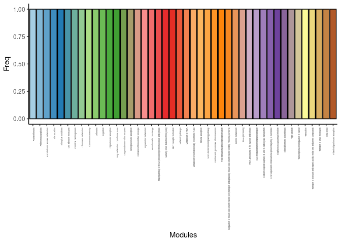
  #dev.off()
  cat("\n \n")
Time by Treatment
count <- count.pathways.traits(time.treat.pathways)[1] 14 [1] 14
Frequency Table
DT.table.freq(count)Frequency Plot
  #pdf("Counts_of_each_pathway_identified_within_jaccard_index.pdf")
  p <- ggplot(data=count,aes(x=list.pathways,y=Freq))
  p <- p + geom_bar(color="black", fill=colorRampPalette(brewer.pal(n = 12, name = "Paired"))(length(count[,1])), stat="identity",position="identity") + theme_classic()
  p <- p + theme(axis.text.x = element_text(angle = 90, hjust =1, size = 3)) + scale_x_discrete(labels=count$list.pathways) + xlab("Modules")
  print(p)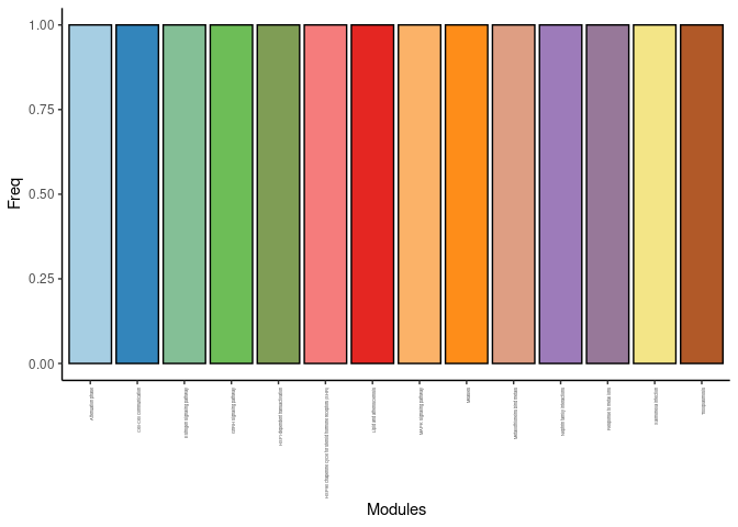
  #dev.off()
  cat("\n \n")
Analysis performed by Ann Wells
The Carter Lab The Jackson Laboratory 2023
ann.wells@jax.org