Module Generation Small Intestine
Ann Wells
April 23, 2023
log.tdata.FPKM.sample.info.subset.small.intestine.WGCNA <- readRDS(here("Data","Small Intestine","log.tdata.FPKM.sample.info.subset.small.intestine.missing.WGCNA.RData"))Set Up Environment
The WGCNA package requires some strict R session environment set up.
options(stringsAsFactors=FALSE)

# Run the following only if running from terminal
# Does NOT work in RStudio
#enableWGCNAThreads()
Choosing Soft-Thresholding Power
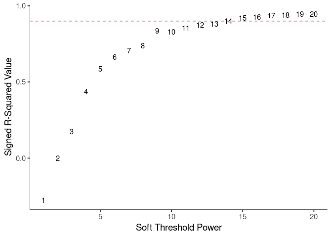
WGCNA uses a smooth softmax function to force a scale-free topology on the gene expression network. I cycled through a set of threshold power values to see which one is the best for the specific topology. As recommended by the authors, I choose the smallest power such that the scale-free topology correlation attempts to hit 0.9.
threshold <- softthreshold(soft)Scale Free Topology
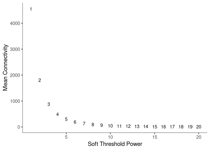
Mean Connectivity
Pick Soft Threshold
knitr::kable(soft$fitIndices)| Power | SFT.R.sq | slope | truncated.R.sq | mean.k. | median.k. | max.k. |
|---|---|---|---|---|---|---|
| 1 | 0.2775045 | 2.7047220 | 0.9818868 | 4554.539174 | 4562.562726 | 6365.1065 |
| 2 | 0.0014650 | 0.0895229 | 0.9598935 | 1810.559844 | 1795.237496 | 3302.1630 |
| 3 | 0.1745212 | -0.7711573 | 0.9546220 | 881.943220 | 856.180669 | 2001.9541 |
| 4 | 0.4378374 | -1.2123772 | 0.9581340 | 487.616279 | 455.803708 | 1330.0345 |
| 5 | 0.5868577 | -1.4341467 | 0.9612379 | 294.371283 | 261.265120 | 939.0257 |
| 6 | 0.6637304 | -1.5769651 | 0.9557433 | 189.650733 | 158.721896 | 692.3847 |
| 7 | 0.7065974 | -1.6313469 | 0.9475429 | 128.477645 | 100.841316 | 527.4167 |
| 8 | 0.7386929 | -1.6181384 | 0.9347663 | 90.592924 | 66.309263 | 412.0482 |
| 9 | 0.8340283 | -1.5439220 | 0.9773235 | 66.004799 | 44.848011 | 332.3930 |
| 10 | 0.8303940 | -1.7436947 | 0.9730376 | 49.420134 | 31.163606 | 300.7217 |
| 11 | 0.8547744 | -1.8493570 | 0.9843070 | 37.867490 | 22.043868 | 274.5585 |
| 12 | 0.8758554 | -1.9162888 | 0.9855476 | 29.596634 | 15.972930 | 252.4468 |
| 13 | 0.8809464 | -1.9685770 | 0.9745136 | 23.533991 | 11.746176 | 233.4278 |
| 14 | 0.9012131 | -1.9659515 | 0.9754621 | 18.997795 | 8.792314 | 216.8406 |
| 15 | 0.9185011 | -1.9527059 | 0.9747652 | 15.541894 | 6.688094 | 202.2120 |
| 16 | 0.9260654 | -1.9465933 | 0.9692790 | 12.866554 | 5.153597 | 189.1921 |
| 17 | 0.9362218 | -1.9232800 | 0.9691979 | 10.765680 | 3.994876 | 177.5155 |
| 18 | 0.9398108 | -1.9075963 | 0.9666279 | 9.094609 | 3.123750 | 166.9757 |
| 19 | 0.9468178 | -1.8822687 | 0.9662150 | 7.749908 | 2.469410 | 157.4093 |
| 20 | 0.9462582 | -1.8659461 | 0.9604304 | 6.656379 | 1.962445 | 148.6846 |
soft$fitIndices %>%
  download_this(
    output_name = "Soft Threshold Small Intestine",
    output_extension = ".csv",
    button_label = "Download data as csv",
    button_type = "info",
    has_icon = TRUE,
    icon = "fa fa-save"
)Calculate Adjacency Matrix and Topological Overlap Matrix
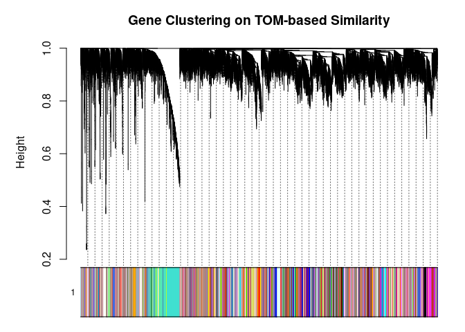
I generated a weighted adjacency matrix for the gene expression profile network using the softmax threshold I determined in the previous step. Then I generate the Topological Overlap Matrix (TOM) for the adjacency matrix. This reduces noise and spurious associations according to the authors.I use the TOM matrix to cluster the profiles of each metabolite based on their similarity. I use dynamic tree cutting to generate modules.
soft.power <- which(soft$fitIndices$SFT.R.sq >= 0.88)[1]
cat("\n", "Power chosen")
##
## Power chosensoft.power## [1] 13cat("\n \n")adj.mtx <- adjacency(log.tdata.FPKM.sample.info.subset.small.intestine.WGCNA, power=soft.power)
TOM = TOMsimilarity(adj.mtx)## ..connectivity..
## ..matrix multiplication (system BLAS)..
## ..normalization..
## ..done.diss.TOM = 1 - TOM
metabolite.clust <- hclust(as.dist(diss.TOM), method="average")
min.module.size <- 15
modules <- cutreeDynamic(dendro=metabolite.clust, distM=diss.TOM, deepSplit=2, pamRespectsDendro=FALSE, minClusterSize=min.module.size)## ..cutHeight not given, setting it to 0.998 ===> 99% of the (truncated) height range in dendro.
## ..done.# Plot modules
cols <- labels2colors(modules)
table(cols)## cols
## aliceblue antiquewhite antiquewhite1
## 45 38 52
## antiquewhite2 antiquewhite3 antiquewhite4
## 64 28 79
## bisque3 bisque4 black
## 25 92 218
## blanchedalmond blue blue1
## 33 347 41
## blue2 blue3 blue4
## 71 48 56
## blueviolet brown brown1
## 57 315 47
## brown2 brown3 brown4
## 71 41 92
## burlywood burlywood1 chocolate1
## 33 24 28
## chocolate2 chocolate3 chocolate4
## 38 45 53
## coral coral1 coral2
## 65 79 79
## coral3 coral4 cornflowerblue
## 64 52 45
## cornsilk cornsilk2 cyan
## 38 28 164
## darkgoldenrod1 darkgoldenrod3 darkgoldenrod4
## 25 34 41
## darkgreen darkgrey darkmagenta
## 129 128 107
## darkolivegreen darkolivegreen1 darkolivegreen2
## 109 48 57
## darkolivegreen4 darkorange darkorange2
## 71 124 93
## darkred darksalmon darkseagreen
## 130 28 39
## darkseagreen1 darkseagreen2 darkseagreen3
## 46 53 65
## darkseagreen4 darkslateblue darkturquoise
## 79 91 128
## darkviolet deeppink deeppink1
## 70 56 47
## deeppink2 deepskyblue deepskyblue4
## 41 32 23
## dodgerblue3 dodgerblue4 firebrick
## 25 35 42
## firebrick2 firebrick3 firebrick4
## 49 57 71
## floralwhite green green1
## 96 266 29
## green2 green3 green4
## 39 46 53
## greenyellow grey grey60
## 197 157 149
## honeydew honeydew1 hotpink4
## 66 81 25
## indianred indianred1 indianred2
## 35 42 49
## indianred3 indianred4 ivory
## 58 73 97
## khaki4 lavender lavenderblush
## 29 39 46
## lavenderblush1 lavenderblush2 lavenderblush3
## 53 66 81
## lightblue lightblue1 lightblue2
## 25 35 42
## lightblue3 lightblue4 lightcoral
## 49 58 73
## lightcyan lightcyan1 lightgoldenrodyellow
## 151 99 29
## lightgreen lightpink lightpink1
## 141 39 46
## lightpink2 lightpink3 lightpink4
## 53 67 82
## lightskyblue1 lightskyblue2 lightskyblue3
## 25 35 42
## lightskyblue4 lightslateblue lightsteelblue
## 49 59 73
## lightsteelblue1 lightyellow linen
## 99 141 30
## magenta magenta1 magenta2
## 208 39 47
## magenta3 magenta4 maroon
## 54 67 82
## mediumorchid mediumorchid2 mediumorchid3
## 78 26 36
## mediumorchid4 mediumpurple mediumpurple1
## 42 49 61
## mediumpurple2 mediumpurple3 mediumpurple4
## 74 99 64
## midnightblue mistyrose mistyrose2
## 162 51 16
## mistyrose3 mistyrose4 moccasin
## 30 39 47
## navajowhite navajowhite1 navajowhite2
## 54 68 84
## navajowhite3 navajowhite4 oldlace
## 45 38 28
## orange orange2 orange3
## 125 26 37
## orange4 orangered orangered1
## 43 50 62
## orangered3 orangered4 paleturquoise
## 74 101 114
## paleturquoise1 paleturquoise3 paleturquoise4
## 20 31 39
## palevioletred palevioletred1 palevioletred2
## 47 54 69
## palevioletred3 peru pink
## 84 27 217
## pink1 pink2 pink3
## 37 43 51
## pink4 plum plum1
## 62 75 103
## plum2 plum3 plum4
## 89 70 56
## powderblue purple purple2
## 47 199 40
## red red1 red4
## 261 32 22
## rosybrown3 rosybrown4 royalblue
## 21 32 135
## royalblue2 royalblue3 saddlebrown
## 40 47 116
## salmon salmon1 salmon2
## 175 55 69
## salmon4 seashell4 sienna
## 87 27 37
## sienna1 sienna2 sienna3
## 43 51 105
## sienna4 skyblue skyblue1
## 63 121 76
## skyblue2 skyblue3 skyblue4
## 77 103 64
## slateblue slateblue1 slateblue2
## 51 45 38
## slateblue3 steelblue steelblue4
## 27 115 21
## tan tan1 tan2
## 177 32 40
## tan3 tan4 thistle
## 47 55 69
## thistle1 thistle2 thistle3
## 87 88 70
## thistle4 tomato tomato2
## 55 47 40
## tomato4 turquoise turquoise2
## 32 1298 22
## violet wheat1 wheat3
## 113 27 38
## white whitesmoke yellow
## 122 44 289
## yellow2 yellow3 yellow4
## 51 63 77
## yellowgreen
## 104plotDendroAndColors(
metabolite.clust, cols, xlab="", sub="", main="Gene Clustering on TOM-based Similarity",
dendroLabels=FALSE, hang=0.03, addGuide=TRUE, guideHang=0.05
)
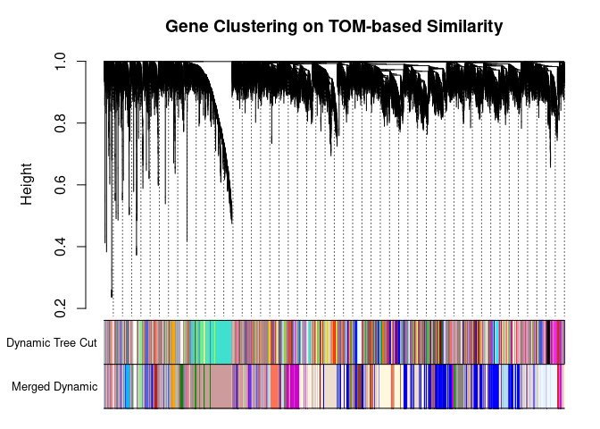
Merging Related Modules
Some modules might be highly correlated. The authors recommend merging modules with a correlation greater than 0.75.
me.list <- moduleEigengenes(log.tdata.FPKM.sample.info.subset.small.intestine.WGCNA, colors=cols)
me <- me.list$eigengenes

# Eigenmetabolite dissimilarity
me.diss <- 1 - cor(me)

h <- hclust(as.dist(me.diss), method="average")

# Merge threshold = 1 - correlation threshold
merge.thresh <- 0.25

plot(h, main="Clustering of Module Eigengene", xlab="", sub="")
abline(h=merge.thresh, col="red")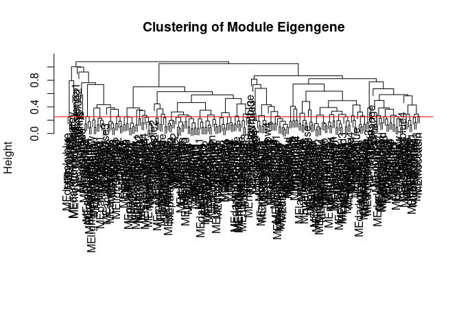
merge <- mergeCloseModules(log.tdata.FPKM.sample.info.subset.small.intestine.WGCNA, cols, cutHeight=merge.thresh, verbose=0)
merged.cols <- merge$colors
merged.mes <- merge$newMEs

  # Check how the merging changed the clustering of the metabolites
plotDendroAndColors(
  metabolite.clust, cbind(cols, merged.cols), c("Dynamic Tree Cut", "Merged Dynamic"), xlab="", sub="",
  main="Gene Clustering on TOM-based Similarity",
  dendroLabels=FALSE, hang=0.03, addGuide=TRUE, guideHang=0.05
  )
Calculating Intramodular Connectivity
This function in WGCNA calculates the total connectivity of a node (metabolite) in the network. The kTotal column specifies this connectivity. The kWithin column specifies the node connectivity within its module. The kOut column specifies the difference between kTotal and kWithin. Generally, the out degree should be lower than the within degree, since the WGCNA procedure groups similar metabolite profiles together.
net.deg <- intramodularConnectivity(adj.mtx, merged.cols)
saveRDS(net.deg,here("Data","Small Intestine","Chang_2DG_BL6_connectivity_small_intestine.RData"))
head(net.deg)
## kTotal kWithin kOut kDiff
## ENSMUSG00000000001 90.513407 41.223547 49.289860 -8.066313
## ENSMUSG00000000028 6.444553 1.535123 4.909430 -3.374307
## ENSMUSG00000000031 4.746692 2.945077 1.801614 1.143463
## ENSMUSG00000000037 4.544815 3.522857 1.021958 2.500899
## ENSMUSG00000000049 2.573566 0.222242 2.351324 -2.129082
## ENSMUSG00000000056 34.562606 22.915767 11.646840 11.268927Summary
The dataset generated coexpression modules of the following sizes. The grey submodule represents metabolites that did not fit well into any of the modules.
table(merged.cols)## merged.cols
## aliceblue antiquewhite antiquewhite1 antiquewhite2 antiquewhite4
## 1423 73 411 1527 303
## blue1 blue2 blue3 burlywood chocolate3
## 1951 319 1072 650 45
## coral1 coral4 cornsilk darkgoldenrod4 deepskyblue
## 765 341 2259 41 213
## firebrick firebrick3 green4 grey hotpink4
## 217 57 467 157 158
## indianred lightblue lightblue2 lightblue4 lightgreen
## 74 25 555 58 141
## lightskyblue2 linen magenta2 magenta3 mediumpurple1
## 35 30 110 710 61
## mediumpurple3 mistyrose moccasin oldlace orange
## 99 51 47 28 125
## pink2 red4 rosybrown3 rosybrown4 royalblue
## 43 22 1532 136 135
## sienna1 sienna3 slateblue2 thistle2 white
## 43 393 116 88 122
## yellow4
## 77# Module names in descending order of size
module.labels <- names(table(merged.cols))[order(table(merged.cols), decreasing=T)]
# Order eigenmetabolites by module labels
merged.mes <- merged.mes[,paste0("ME", module.labels)]
colnames(merged.mes) <- paste0("log.tdata.FPKM.sample.info.subset.small.intestine.WGCNA_", module.labels)
module.eigens <- merged.mes
# Add log.tdata.FPKM.sample.info.subset.WGCNA tag to labels
module.labels <- paste0("log.tdata.FPKM.sample.info.subset.small.intestine.WGCNA_", module.labels)
# Generate and store metabolite membership
module.membership <- data.frame(
Gene=colnames(log.tdata.FPKM.sample.info.subset.small.intestine.WGCNA),
Module=paste0("log.tdata.FPKM.sample.info.subset.small.intestine.WGCNA_", merged.cols)
)
saveRDS(module.labels, here("Data","Small Intestine","log.tdata.FPKM.sample.info.subset.small.intestine.WGCNA.module.labels.RData"))
saveRDS(module.eigens, here("Data","Small Intestine","log.tdata.FPKM.sample.info.subset.small.intestine.WGCNA.module.eigens.RData"))
saveRDS(module.membership, here("Data","Small Intestine", "log.tdata.FPKM.sample.info.subset.small.intestine.WGCNA.module.membership.RData"))
write.table(module.labels, here("Data","Small Intestine","log.tdata.FPKM.sample.info.subset.small.intestine.WGCNA.module.labels.csv"), row.names=F, col.names=F, sep=",")
write.csv(module.eigens, here("Data","Small Intestine","log.tdata.FPKM.sample.info.subset.small.intestine.WGCNA.module.eigens.csv"))
write.csv(module.membership, here("Data","Small Intestine","log.tdata.FPKM.sample.info.subset.small.intestine.WGCNA.module.membership.csv"), row.names=F)Analysis performed by Ann Wells
The Carter Lab The Jackson Laboratory 2023
ann.wells@jax.org