Module Generation Kidney
Ann Wells
April 23, 2023
log.tdata.FPKM.sample.info.subset.kidney.WGCNA <- readRDS(here("Data","Kidney","log.tdata.FPKM.sample.info.subset.kidney.missing.WGCNA.RData"))Set Up Environment
The WGCNA package requires some strict R session environment set up.
options(stringsAsFactors=FALSE)

# Run the following only if running from terminal
# Does NOT work in RStudio
#enableWGCNAThreads()
Choosing Soft-Thresholding Power
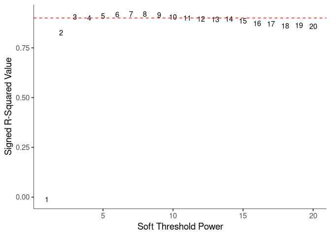
WGCNA uses a smooth softmax function to force a scale-free topology on the gene expression network. I cycled through a set of threshold power values to see which one is the best for the specific topology. As recommended by the authors, I choose the smallest power such that the scale-free topology correlation attempts to hit 0.9.
threshold <- softthreshold(soft)Scale Free Topology
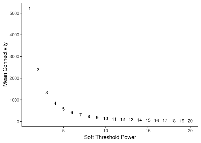
Mean Connectivity
Pick Soft Threshold
knitr::kable(soft$fitIndices)| Power | SFT.R.sq | slope | truncated.R.sq | mean.k. | median.k. | max.k. |
|---|---|---|---|---|---|---|
| 1 | 0.0121149 | 0.1191019 | 0.1004789 | 5219.32881 | 5030.021248 | 8138.1306 |
| 2 | 0.8269769 | -0.7247705 | 0.8027802 | 2400.04106 | 2054.401979 | 5261.4865 |
| 3 | 0.9047741 | -0.9281069 | 0.8839740 | 1346.37199 | 988.355279 | 3849.4411 |
| 4 | 0.9000023 | -1.0102613 | 0.8838498 | 848.96011 | 522.210252 | 3002.0491 |
| 5 | 0.9102486 | -1.0494899 | 0.9042740 | 577.73461 | 295.401073 | 2433.7416 |
| 6 | 0.9167395 | -1.0744289 | 0.9200976 | 414.66085 | 175.175676 | 2025.2100 |
| 7 | 0.9207505 | -1.0969138 | 0.9327132 | 309.48819 | 107.994902 | 1717.4162 |
| 8 | 0.9193461 | -1.1130551 | 0.9401131 | 238.00293 | 70.132323 | 1477.5613 |
| 9 | 0.9141197 | -1.1386159 | 0.9410161 | 187.40248 | 47.002239 | 1288.9178 |
| 10 | 0.9062091 | -1.1608965 | 0.9410373 | 150.41174 | 32.456281 | 1136.5033 |
| 11 | 0.8995423 | -1.1812848 | 0.9433819 | 122.65231 | 22.590468 | 1010.1775 |
| 12 | 0.8946226 | -1.2014140 | 0.9437366 | 101.36322 | 16.091618 | 904.0374 |
| 13 | 0.8929483 | -1.2148416 | 0.9461115 | 84.73491 | 11.702673 | 813.8259 |
| 14 | 0.8945988 | -1.2296059 | 0.9503828 | 71.54233 | 8.728525 | 736.3938 |
| 15 | 0.8864482 | -1.2494851 | 0.9481451 | 60.93305 | 6.538767 | 669.3603 |
| 16 | 0.8740652 | -1.2726779 | 0.9403562 | 52.29964 | 4.989716 | 610.8924 |
| 17 | 0.8703653 | -1.2898556 | 0.9410834 | 45.20035 | 3.840544 | 559.5562 |
| 18 | 0.8600518 | -1.3074938 | 0.9366588 | 39.30803 | 3.002556 | 514.2143 |
| 19 | 0.8630285 | -1.3187056 | 0.9412918 | 34.37652 | 2.342548 | 473.9535 |
| 20 | 0.8586851 | -1.3346929 | 0.9412695 | 30.21798 | 1.850999 | 438.0323 |
soft$fitIndices %>%
  download_this(
    output_name = "Soft Threshold Kidney",
    output_extension = ".csv",
    button_label = "Download data as csv",
    button_type = "info",
    has_icon = TRUE,
    icon = "fa fa-save"
)Calculate Adjacency Matrix and Topological Overlap Matrix
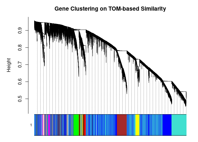
I generated a weighted adjacency matrix for the gene expression profile network using the softmax threshold I determined in the previous step. Then I generate the Topological Overlap Matrix (TOM) for the adjacency matrix. This reduces noise and spurious associations according to the authors.I use the TOM matrix to cluster the profiles of each metabolite based on their similarity. I use dynamic tree cutting to generate modules.
soft.power <- which(soft$fitIndices$SFT.R.sq >= 0.88)[1]
cat("\n", "Power chosen")
##
## Power chosensoft.power## [1] 3cat("\n \n")adj.mtx <- adjacency(log.tdata.FPKM.sample.info.subset.kidney.WGCNA, power=soft.power)
TOM = TOMsimilarity(adj.mtx)## ..connectivity..
## ..matrix multiplication (system BLAS)..
## ..normalization..
## ..done.diss.TOM = 1 - TOM
metabolite.clust <- hclust(as.dist(diss.TOM), method="average")
min.module.size <- 15
modules <- cutreeDynamic(dendro=metabolite.clust, distM=diss.TOM, deepSplit=2, pamRespectsDendro=FALSE, minClusterSize=min.module.size)## ..cutHeight not given, setting it to 0.953 ===> 99% of the (truncated) height range in dendro.
## ..done.# Plot modules
cols <- labels2colors(modules)
table(cols)## cols
## black blue brown cyan darkgreen
## 376 5955 1169 78 26
## darkgrey darkred darkturquoise green greenyellow
## 19 33 23 575 93
## grey60 lightcyan lightgreen lightyellow magenta
## 59 62 47 43 141
## midnightblue pink purple red royalblue
## 63 240 98 415 37
## salmon tan turquoise yellow
## 80 86 6794 743plotDendroAndColors(
metabolite.clust, cols, xlab="", sub="", main="Gene Clustering on TOM-based Similarity",
dendroLabels=FALSE, hang=0.03, addGuide=TRUE, guideHang=0.05
)
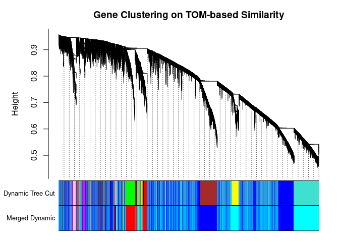
Merging Related Modules
Some modules might be highly correlated. The authors recommend merging modules with a correlation greater than 0.75.
me.list <- moduleEigengenes(log.tdata.FPKM.sample.info.subset.kidney.WGCNA, colors=cols)
me <- me.list$eigengenes

# Eigenmetabolite dissimilarity
me.diss <- 1 - cor(me)

h <- hclust(as.dist(me.diss), method="average")

# Merge threshold = 1 - correlation threshold
merge.thresh <- 0.25

plot(h, main="Clustering of Module Eigengene", xlab="", sub="")
abline(h=merge.thresh, col="red")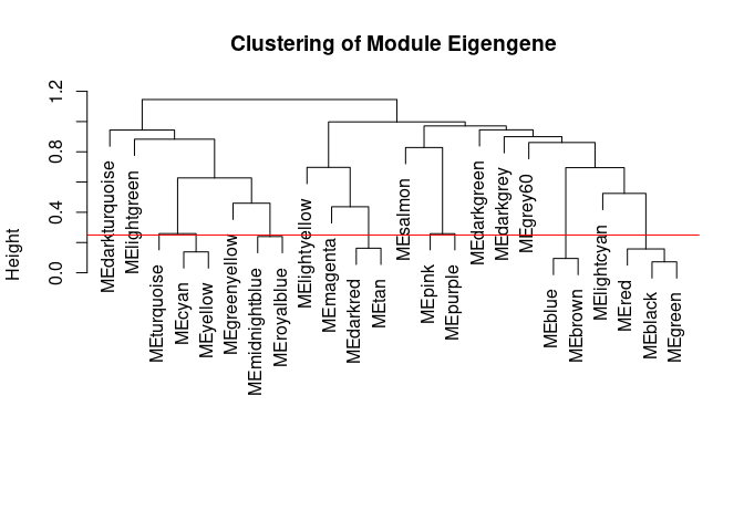
merge <- mergeCloseModules(log.tdata.FPKM.sample.info.subset.kidney.WGCNA, cols, cutHeight=merge.thresh, verbose=0)
merged.cols <- merge$colors
merged.mes <- merge$newMEs

  # Check how the merging changed the clustering of the metabolites
plotDendroAndColors(
  metabolite.clust, cbind(cols, merged.cols), c("Dynamic Tree Cut", "Merged Dynamic"), xlab="", sub="",
  main="Gene Clustering on TOM-based Similarity",
  dendroLabels=FALSE, hang=0.03, addGuide=TRUE, guideHang=0.05
  )
Calculating Intramodular Connectivity
This function in WGCNA calculates the total connectivity of a node (metabolite) in the network. The kTotal column specifies this connectivity. The kWithin column specifies the node connectivity within its module. The kOut column specifies the difference between kTotal and kWithin. Generally, the out degree should be lower than the within degree, since the WGCNA procedure groups similar metabolite profiles together.
net.deg <- intramodularConnectivity(adj.mtx, merged.cols)
saveRDS(net.deg,here("Data","Kidney","Chang_2DG_BL6_connectivity_kidney.RData"))
head(net.deg)
## kTotal kWithin kOut kDiff
## ENSMUSG00000000001 1252.6918 16.5587 1236.1331 -1219.57435
## ENSMUSG00000000028 271.4714 106.9441 164.5272 -57.58306
## ENSMUSG00000000031 244.8089 105.1601 139.6488 -34.48862
## ENSMUSG00000000037 363.2693 158.4235 204.8458 -46.42233
## ENSMUSG00000000049 679.5418 408.0787 271.4631 136.61559
## ENSMUSG00000000056 508.8386 237.7036 271.1350 -33.43135Summary
The dataset generated coexpression modules of the following sizes. The grey submodule represents metabolites that did not fit well into any of the modules.
table(merged.cols)## merged.cols
## blue cyan darkgreen darkgrey darkred
## 7124 7615 26 19 119
## darkturquoise greenyellow grey60 lightcyan lightgreen
## 23 93 59 62 47
## lightyellow magenta midnightblue pink purple
## 43 141 100 240 98
## red salmon
## 1366 80# Module names in descending order of size
module.labels <- names(table(merged.cols))[order(table(merged.cols), decreasing=T)]
# Order eigenmetabolites by module labels
merged.mes <- merged.mes[,paste0("ME", module.labels)]
colnames(merged.mes) <- paste0("log.tdata.FPKM.sample.info.subset.kidney.WGCNA_", module.labels)
module.eigens <- merged.mes
# Add log.tdata.FPKM.sample.info.subset.WGCNA tag to labels
module.labels <- paste0("log.tdata.FPKM.sample.info.subset.kidney.WGCNA_", module.labels)
# Generate and store metabolite membership
module.membership <- data.frame(
Gene=colnames(log.tdata.FPKM.sample.info.subset.kidney.WGCNA),
Module=paste0("log.tdata.FPKM.sample.info.subset.kidney.WGCNA_", merged.cols)
)
saveRDS(module.labels, here("Data","Kidney","log.tdata.FPKM.sample.info.subset.kidney.WGCNA.module.labels.RData"))
saveRDS(module.eigens, here("Data","Kidney","log.tdata.FPKM.sample.info.subset.kidney.WGCNA.module.eigens.RData"))
saveRDS(module.membership, here("Data","Kidney", "log.tdata.FPKM.sample.info.subset.kidney.WGCNA.module.membership.RData"))
write.table(module.labels, here("Data","Kidney","log.tdata.FPKM.sample.info.subset.kidney.WGCNA.module.labels.csv"), row.names=F, col.names=F, sep=",")
write.csv(module.eigens, here("Data","Kidney","log.tdata.FPKM.sample.info.subset.kidney.WGCNA.module.eigens.csv"))
write.csv(module.membership, here("Data","Kidney","log.tdata.FPKM.sample.info.subset.kidney.WGCNA.module.membership.csv"), row.names=F)Analysis performed by Ann Wells
The Carter Lab The Jackson Laboratory 2023
ann.wells@jax.org