Module Generation Hypothalamus
Ann Wells
April 23, 2023
log.tdata.FPKM.sample.info.subset.hypothalamus.WGCNA <- readRDS(here("Data","Hypothalamus","log.tdata.FPKM.sample.info.subset.hypothalamus.missing.WGCNA.RData"))Set Up Environment
The WGCNA package requires some strict R session environment set up.
options(stringsAsFactors=FALSE)

# Run the following only if running from terminal
# Does NOT work in RStudio
#enableWGCNAThreads()
Choosing Soft-Thresholding Power
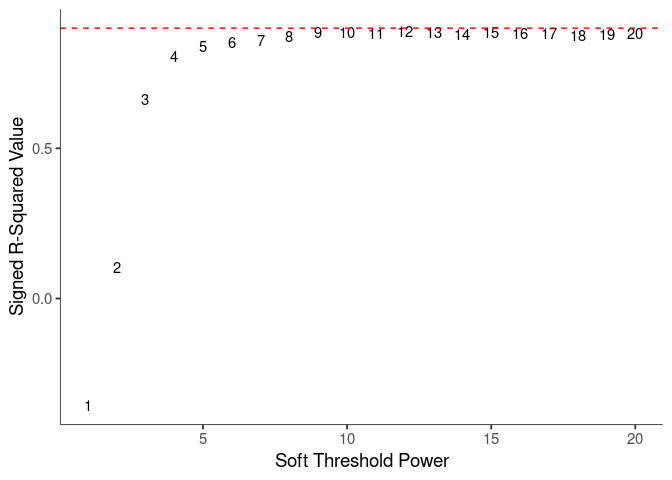
WGCNA uses a smooth softmax function to force a scale-free topology on the gene expression network. I cycled through a set of threshold power values to see which one is the best for the specific topology. As recommended by the authors, I choose the smallest power such that the scale-free topology correlation attempts to hit 0.9.
threshold <- softthreshold(soft)Scale Free Topology
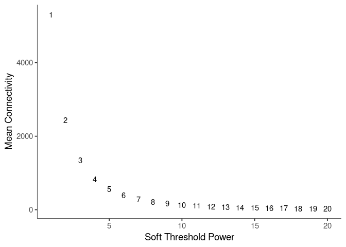
Mean Connectivity
Pick Soft Threshold
knitr::kable(soft$fitIndices)| Power | SFT.R.sq | slope | truncated.R.sq | mean.k. | median.k. | max.k. |
|---|---|---|---|---|---|---|
| 1 | 0.3572320 | 1.4608066 | 0.8432363 | 5311.78071 | 5285.004944 | 7872.2853 |
| 2 | 0.1042735 | -0.2841925 | 0.7996520 | 2429.97913 | 2280.856205 | 4909.0908 |
| 3 | 0.6623934 | -0.7875397 | 0.9043205 | 1342.72698 | 1155.231987 | 3476.8795 |
| 4 | 0.8045534 | -0.9962505 | 0.9276023 | 830.47967 | 645.467420 | 2636.7361 |
| 5 | 0.8399950 | -1.1128797 | 0.9282658 | 553.76111 | 384.647264 | 2087.1171 |
| 6 | 0.8535998 | -1.1833409 | 0.9314950 | 389.62589 | 240.731083 | 1701.6497 |
| 7 | 0.8585690 | -1.2324981 | 0.9322639 | 285.41431 | 156.899351 | 1417.9707 |
| 8 | 0.8734672 | -1.2599093 | 0.9444936 | 215.73691 | 104.970641 | 1201.6904 |
| 9 | 0.8863359 | -1.2812215 | 0.9539879 | 167.21828 | 72.444878 | 1032.3886 |
| 10 | 0.8846802 | -1.3038105 | 0.9543299 | 132.30884 | 50.926875 | 897.4662 |
| 11 | 0.8814863 | -1.3239066 | 0.9528432 | 106.50525 | 36.424692 | 787.5637 |
| 12 | 0.8875035 | -1.3337608 | 0.9592374 | 86.99682 | 26.493157 | 696.7081 |
| 13 | 0.8853058 | -1.3448866 | 0.9600692 | 71.96189 | 19.632679 | 620.6496 |
| 14 | 0.8789485 | -1.3612654 | 0.9576409 | 60.18147 | 14.694100 | 556.2865 |
| 15 | 0.8845999 | -1.3685519 | 0.9630346 | 50.81721 | 11.137944 | 501.3044 |
| 16 | 0.8807653 | -1.3801481 | 0.9606901 | 43.27874 | 8.584439 | 453.9445 |
| 17 | 0.8828753 | -1.3892138 | 0.9625452 | 37.14158 | 6.668277 | 412.8480 |
| 18 | 0.8768878 | -1.4043292 | 0.9599819 | 32.09490 | 5.219548 | 376.9500 |
| 19 | 0.8792290 | -1.4072977 | 0.9630983 | 27.90735 | 4.116817 | 345.4055 |
| 20 | 0.8806498 | -1.4114030 | 0.9657176 | 24.40424 | 3.285183 | 317.5362 |
soft$fitIndices %>%
  download_this(
    output_name = "Soft Threshold Hypothalamus",
    output_extension = ".csv",
    button_label = "Download data as csv",
    button_type = "info",
    has_icon = TRUE,
    icon = "fa fa-save"
)Calculate Adjacency Matrix and Topological Overlap Matrix
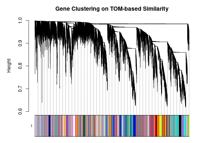
I generated a weighted adjacency matrix for the gene expression profile network using the softmax threshold I determined in the previous step. Then I generate the Topological Overlap Matrix (TOM) for the adjacency matrix. This reduces noise and spurious associations according to the authors.I use the TOM matrix to cluster the profiles of each metabolite based on their similarity. I use dynamic tree cutting to generate modules.
soft.power <- which(soft$fitIndices$SFT.R.sq >= 0.88)[1]
cat("\n", "Power chosen")
##
## Power chosensoft.power## [1] 9cat("\n \n")adj.mtx <- adjacency(log.tdata.FPKM.sample.info.subset.hypothalamus.WGCNA, power=soft.power)
TOM = TOMsimilarity(adj.mtx)## ..connectivity..
## ..matrix multiplication (system BLAS)..
## ..normalization..
## ..done.diss.TOM = 1 - TOM
metabolite.clust <- hclust(as.dist(diss.TOM), method="average")
min.module.size <- 15
modules <- cutreeDynamic(dendro=metabolite.clust, distM=diss.TOM, deepSplit=2, pamRespectsDendro=FALSE, minClusterSize=min.module.size)## ..cutHeight not given, setting it to 0.996 ===> 99% of the (truncated) height range in dendro.
## ..done.# Plot modules
cols <- labels2colors(modules)
table(cols)## cols
## antiquewhite2 antiquewhite4 bisque4 black blue
## 46 83 108 510 1162
## blue2 brown brown2 brown4 coral
## 60 846 62 109 47
## coral1 coral2 coral3 cyan darkgreen
## 83 81 46 269 204
## darkgrey darkmagenta darkolivegreen darkolivegreen4 darkorange
## 188 149 151 63 181
## darkorange2 darkred darkseagreen3 darkseagreen4 darkslateblue
## 111 211 48 86 108
## darkturquoise darkviolet firebrick4 floralwhite green
## 201 59 63 113 602
## greenyellow grey grey60 honeydew honeydew1
## 315 98 235 49 88
## indianred4 ivory lavenderblush2 lavenderblush3 lightblue4
## 65 115 50 89 23
## lightcoral lightcyan lightcyan1 lightgreen lightpink3
## 68 238 118 226 50
## lightpink4 lightslateblue lightsteelblue lightsteelblue1 lightyellow
## 93 27 70 120 222
## magenta magenta4 maroon mediumorchid mediumpurple1
## 439 51 93 78 30
## mediumpurple2 mediumpurple3 mediumpurple4 midnightblue navajowhite1
## 71 122 42 252 52
## navajowhite2 orange orangered1 orangered3 orangered4
## 94 186 31 73 125
## paleturquoise palevioletred2 palevioletred3 pink pink4
## 166 58 96 496 37
## plum plum1 plum2 plum3 purple
## 73 129 105 58 406
## red royalblue saddlebrown salmon salmon2
## 537 214 173 291 58
## salmon4 sienna3 sienna4 skyblue skyblue1
## 97 145 39 175 75
## skyblue2 skyblue3 skyblue4 steelblue tan
## 78 138 42 166 299
## thistle thistle1 thistle2 thistle3 turquoise
## 58 102 103 58 1345
## violet white yellow yellow3 yellow4
## 156 179 760 40 75
## yellowgreen
## 139plotDendroAndColors(
metabolite.clust, cols, xlab="", sub="", main="Gene Clustering on TOM-based Similarity",
dendroLabels=FALSE, hang=0.03, addGuide=TRUE, guideHang=0.05
)
Merging Related Modules
Some modules might be highly correlated. The authors recommend merging modules with a correlation greater than 0.75.
me.list <- moduleEigengenes(log.tdata.FPKM.sample.info.subset.hypothalamus.WGCNA, colors=cols)
me <- me.list$eigengenes

# Eigenmetabolite dissimilarity
me.diss <- 1 - cor(me)

h <- hclust(as.dist(me.diss), method="average")

# Merge threshold = 1 - correlation threshold
merge.thresh <- 0.25

plot(h, main="Clustering of Module Eigengene", xlab="", sub="")
abline(h=merge.thresh, col="red")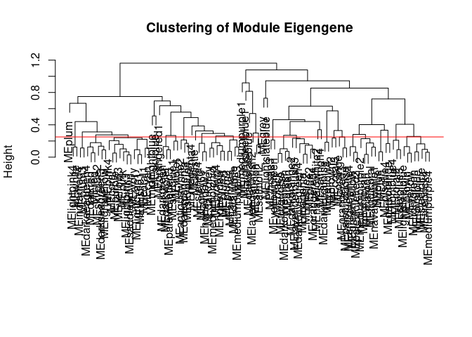
merge <- mergeCloseModules(log.tdata.FPKM.sample.info.subset.hypothalamus.WGCNA, cols, cutHeight=merge.thresh, verbose=0)
merged.cols <- merge$colors
merged.mes <- merge$newMEs
# Check how the merging changed the clustering of the metabolites
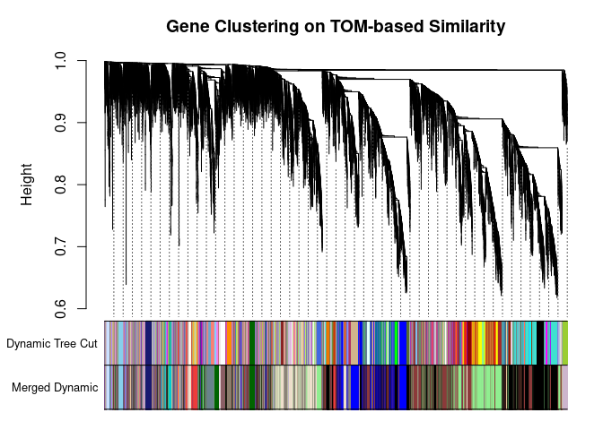
plotDendroAndColors(
metabolite.clust, cbind(cols, merged.cols), c("Dynamic Tree Cut", "Merged Dynamic"), xlab="", sub="",
main="Gene Clustering on TOM-based Similarity",
dendroLabels=FALSE, hang=0.03, addGuide=TRUE, guideHang=0.05
)
Calculating Intramodular Connectivity
This function in WGCNA calculates the total connectivity of a node (metabolite) in the network. The kTotal column specifies this connectivity. The kWithin column specifies the node connectivity within its module. The kOut column specifies the difference between kTotal and kWithin. Generally, the out degree should be lower than the within degree, since the WGCNA procedure groups similar metabolite profiles together.
net.deg <- intramodularConnectivity(adj.mtx, merged.cols)
saveRDS(net.deg,here("Data","Hypothalamus","Chang_2DG_BL6_connectivity_hypothalamus.RData"))
head(net.deg)
## kTotal kWithin kOut kDiff
## ENSMUSG00000000001 446.682428 181.951383 264.731045 -82.779662
## ENSMUSG00000000028 30.953292 18.080976 12.872316 5.208660
## ENSMUSG00000000031 15.022966 5.064422 9.958544 -4.894122
## ENSMUSG00000000037 199.423312 52.333495 147.089817 -94.756322
## ENSMUSG00000000049 13.502491 5.997018 7.505472 -1.508454
## ENSMUSG00000000056 9.084321 3.587350 5.496972 -1.909622Summary
The dataset generated coexpression modules of the following sizes. The grey submodule represents metabolites that did not fit well into any of the modules.
table(merged.cols)## merged.cols
## antiquewhite2 antiquewhite4 bisque4 black blue
## 1746 978 289 3598 1461
## brown2 darkgreen darkslateblue darkturquoise grey
## 533 590 108 276 98
## indianred4 lavenderblush2 lightblue4 lightgreen lightpink4
## 3241 50 591 2387 272
## lightslateblue lightsteelblue1 mediumpurple1 midnightblue navajowhite2
## 27 120 30 252 94
## orangered1 plum salmon4 skyblue thistle3
## 31 73 97 175 197# Module names in descending order of size
module.labels <- names(table(merged.cols))[order(table(merged.cols), decreasing=T)]
# Order eigenmetabolites by module labels
merged.mes <- merged.mes[,paste0("ME", module.labels)]
colnames(merged.mes) <- paste0("log.tdata.FPKM.sample.info.subset.hypothalamus.WGCNA_", module.labels)
module.eigens <- merged.mes
# Add log.tdata.FPKM.sample.info.subset.WGCNA tag to labels
module.labels <- paste0("log.tdata.FPKM.sample.info.subset.hypothalamus.WGCNA_", module.labels)
# Generate and store metabolite membership
module.membership <- data.frame(
Gene=colnames(log.tdata.FPKM.sample.info.subset.hypothalamus.WGCNA),
Module=paste0("log.tdata.FPKM.sample.info.subset.hypothalamus.WGCNA_", merged.cols)
)
saveRDS(module.labels, here("Data","Hypothalamus","log.tdata.FPKM.sample.info.subset.hypothalamus.WGCNA.module.labels.RData"))
saveRDS(module.eigens, here("Data","Hypothalamus","log.tdata.FPKM.sample.info.subset.hypothalamus.WGCNA.module.eigens.RData"))
saveRDS(module.membership, here("Data","Hypothalamus", "log.tdata.FPKM.sample.info.subset.hypothalamus.WGCNA.module.membership.RData"))
write.table(module.labels, here("Data","Hypothalamus","log.tdata.FPKM.sample.info.subset.hypothalamus.WGCNA.module.labels.csv"), row.names=F, col.names=F, sep=",")
write.csv(module.eigens, here("Data","Hypothalamus","log.tdata.FPKM.sample.info.subset.hypothalamus.WGCNA.module.eigens.csv"))
write.csv(module.membership, here("Data","Hypothalamus","log.tdata.FPKM.sample.info.subset.hypothalamus.WGCNA.module.membership.csv"), row.names=F)Analysis performed by Ann Wells
The Carter Lab The Jackson Laboratory 2023
ann.wells@jax.org