Contribution of Main Effects Liver
Ann Wells
April 23, 2023
Introduction and Data files
This dataset contains nine tissues (heart, hippocampus, hypothalamus, kidney, liver, prefrontal cortex, skeletal muscle, small intestine, and spleen) from C57BL/6J mice that were fed 2-deoxyglucose (6g/L) through their drinking water for 96hrs or 4wks. 96hr mice were given their 2DG treatment 2 weeks after the other cohort started the 4 week treatment. The organs from the mice were harvested and processed for metabolomics and transcriptomics. The data in this document pertains to the transcriptomics data only. The counts that were used were FPKM normalized before being log transformed. It was determined that sample A113 had low RNAseq quality and through further analyses with PCA, MA plots, and clustering was an outlier and will be removed for the rest of the analyses performed. This document will determine the contribution of each main effect or their combination to each module identified, as well as the relationship of each gene within the module and its significance.
needed.packages <- c("tidyverse", "here", "functional", "gplots", "dplyr", "GeneOverlap", "R.utils", "reshape2","magrittr","data.table", "RColorBrewer","preprocessCore", "ARTool","emmeans", "phia", "gProfileR", "WGCNA","plotly", "pheatmap","ppcor", "pander","downloadthis")
for(i in 1:length(needed.packages)){library(needed.packages[i], character.only = TRUE)}
source(here("source_files","WGCNA_source.R"))
source(here("source_files","WGCNA_contribution_source.R"))tdata.FPKM.sample.info <- readRDS(here("Data","20190406_RNAseq_B6_4wk_2DG_counts_phenotypes.RData"))
tdata.FPKM <- readRDS(here("Data","20190406_RNAseq_B6_4wk_2DG_counts_numeric.RData"))
log.tdata.FPKM <- log(tdata.FPKM + 1)
log.tdata.FPKM <- as.data.frame(log.tdata.FPKM)
log.tdata.FPKM.sample.info <- cbind(log.tdata.FPKM, tdata.FPKM.sample.info[,27238:27240])
log.tdata.FPKM.sample.info <- log.tdata.FPKM.sample.info %>% rownames_to_column() %>% filter(rowname != "A113") %>% column_to_rownames()
log.tdata.FPKM.subset <- log.tdata.FPKM[,colMeans(log.tdata.FPKM != 0) > 0.5]
log.tdata.FPKM.subset <- log.tdata.FPKM.subset %>% rownames_to_column() %>% filter(rowname != "A113") %>% column_to_rownames()
log.tdata.FPKM.sample.info.subset.liver <- log.tdata.FPKM.sample.info %>% rownames_to_column() %>% filter(Tissue == "Liver") %>% column_to_rownames()
log.tdata.FPKM.subset <- subset(log.tdata.FPKM.sample.info.subset.liver, select = -c(Time,Treatment,Tissue))
WGCNA.pathway <-readRDS(here("Data","Liver","Chang_B6_96hr_4wk_gprofiler_pathway_annotation_list_liver_WGCNA.RData"))
Matched<-readRDS(here("Data","Liver","Annotated_genes_in_liver_WGCNA_Chang_B6_96hr_4wk.RData"))
module.names <- Matched$X..Module.
name <- str_split(module.names,"_")
samples <-c()
for(i in 1:length(name)){
samples[[i]] <- name[[i]][2]
}
name <- str_split(samples,"\"")
name <- unlist(name)
Treatment <- unclass(as.factor(log.tdata.FPKM.sample.info.subset.liver[,27238]))
Time <- unclass(as.factor(log.tdata.FPKM.sample.info.subset.liver[,27237]))
Treat.Time <- paste0(Treatment, Time)
phenotype <- data.frame(cbind(Treatment, Time, Treat.Time))
nSamples <- nrow(log.tdata.FPKM.sample.info.subset.liver)
MEs0 <- read.csv(here("Data","Liver","log.tdata.FPKM.sample.info.subset.liver.WGCNA.module.eigens.csv"),header = T, row.names = 1)
name <- str_split(names(MEs0),"_")
samples <-c()
for(i in 1:length(name)){
samples[[i]] <- name[[i]][2]
}
name <- str_split(samples,"\"")
name <- unlist(name)
colnames(MEs0) <-name
MEs <- orderMEs(MEs0)
moduleTraitCor <- cor(MEs, phenotype, use = "p");
moduleTraitPvalue <- corPvalueStudent(moduleTraitCor, nSamples)Relationship between Modules and Traits
#sizeGrWindow(10,6)
# Will display correlations and their p-values
textMatrix = paste(signif(moduleTraitCor, 2), "\n(",
signif(moduleTraitPvalue, 1), ")", sep = "");
dim(textMatrix) = dim(moduleTraitCor)
# Display the correlation values within a heatmap plot
heat <- pheatmap(moduleTraitCor, main = paste("Module-trait relationships"), color=colorRampPalette(brewer.pal(n = 12, name = "Paired"))(10), cluster_rows = F, cluster_cols = F, fontsize_number = 4, angle_col = 45, number_color = "black", border_color = "white")
heat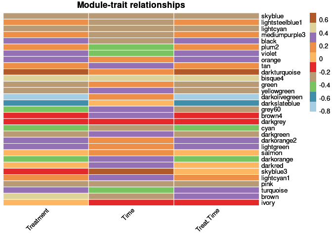
DT::datatable(moduleTraitPvalue, extensions = 'Buttons',
rownames = TRUE,
filter="top",
options = list(dom = 'Blfrtip',
buttons = c('copy', 'csv', 'excel'),
lengthMenu = list(c(10,25,50,-1),
c(10,25,50,"All")),
scrollX= TRUE), class = "display")Partial Correlation
# phenotype$Treatment <- as.numeric(phenotype$Treatment)
# phenotype$Time <- as.numeric(phenotype$Time)
# phenotype$Treat.Time <- as.numeric(phenotype$Treat.Time)
#
# Sigmodules <- as.data.frame(cbind(MEs$darkturquoise,MEs$darkolivegreen,MEs$skyblue3))
# colnames(Sigmodules) <- c("darkturquoise","darkolivegreen","skyblue3")
#
# for(i in 1:length(Sigmodules)){
# cat("\n##",colnames(Sigmodules[i]),"{.tabset .tabset-fade .tabset-pills}","\n")
# for(j in 1:length(phenotype)){
# cat("\n###", colnames(phenotype[j]),"{.tabset .tabset-fade .tabset-pills}","\n")
# for(k in 1:length(phenotype)){
# cat("\n####", "Partial Correlation", colnames(phenotype[k]),"\n")
# partial <- pcor.test(Sigmodules[,i], phenotype[,j],phenotype[,k])
# panderOptions('knitr.auto.asis', FALSE)
# print(pander(partial))
# cat("\n \n")
# }
# cat("\n \n")
# }
# cat("\n \n")
# }Scatterplots Module membership vs. Gene significance
Time
time.contribution(phenotype, log.tdata.FPKM.subset, MEs)skyblue
lightsteelblue1
lightcyan
mediumpurple3
black
plum2
violet
orange
tan
darkturquoise
bisque4
green
yellowgreen
darkolivegreen
darkslateblue
grey60
brown4
darkgrey
cyan
darkgreen
darkorange2
lightgreen
salmon
darkorange
darkred
skyblue3
lightcyan1
pink
turquoise
brown
ivory
Treatment
treat.contribution(phenotype, log.tdata.FPKM.subset, MEs)skyblue
lightsteelblue1
lightcyan
mediumpurple3
black
plum2
violet
orange
tan
darkturquoise
bisque4
green
yellowgreen
darkolivegreen
darkslateblue
grey60
brown4
darkgrey
cyan
darkgreen
darkorange2
lightgreen
salmon
darkorange
darkred
skyblue3
lightcyan1
pink
turquoise
brown
ivory
Treatment by Time
treat.time.contribution(phenotype, log.tdata.FPKM.subset, MEs)skyblue
lightsteelblue1
lightcyan
mediumpurple3
black
plum2
violet
orange
tan
darkturquoise
bisque4
green
yellowgreen
darkolivegreen
darkslateblue
grey60
brown4
darkgrey
cyan
darkgreen
darkorange2
lightgreen
salmon
darkorange
darkred
skyblue3
lightcyan1
pink
turquoise
brown
ivory
Analysis performed by Ann Wells
The Carter Lab The Jackson Laboratory 2023
ann.wells@jax.org