Module Generation SM.SI.spleen
Ann Wells
April 23, 2023
log.tdata.FPKM.sample.info.subset.SM.SI.spleen.WGCNA <- readRDS(here("Data","SM.SI.spleen","log.tdata.FPKM.sample.info.subset.SM.SI.spleen.missing.WGCNA.RData"))Set Up Environment
The WGCNA package requires some strict R session environment set up.
options(stringsAsFactors=FALSE)

# Run the following only if running from terminal
# Does NOT work in RStudio
#enableWGCNAThreads()
Choosing Soft-Thresholding Power
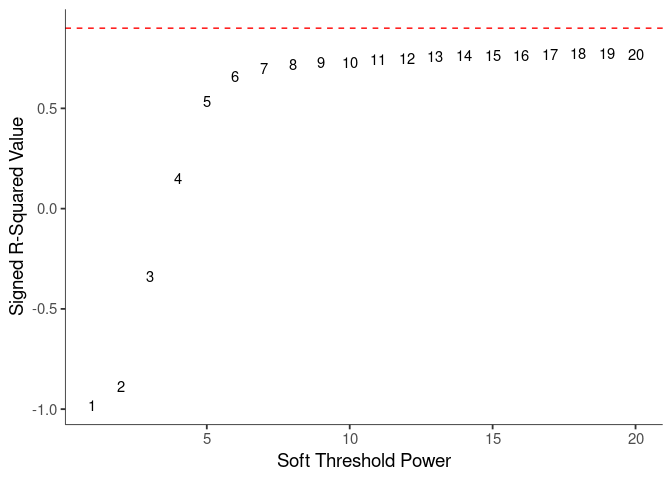
WGCNA uses a smooth softmax function to force a scale-free topology on the gene expression network. I cycled through a set of threshold power values to see which one is the best for the specific topology. As recommended by the authors, I choose the smallest power such that the scale-free topology correlation attempts to hit 0.9.
threshold <- softthreshold(soft)Scale Free Topology
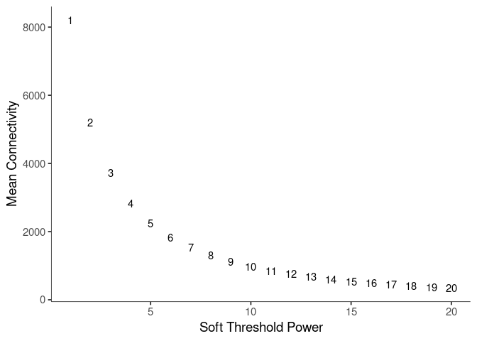
Mean Connectivity
Pick Soft Threshold
knitr::kable(soft$fitIndices)| Power | SFT.R.sq | slope | truncated.R.sq | mean.k. | median.k. | max.k. |
|---|---|---|---|---|---|---|
| 1 | 0.9834138 | 1.8131280 | 0.9799078 | 8208.3139 | 8779.6491 | 11036.802 |
| 2 | 0.8846923 | 0.5517303 | 0.8876201 | 5203.0387 | 5523.0568 | 8407.821 |
| 3 | 0.3391311 | 0.1376277 | 0.2423267 | 3713.4777 | 3815.9326 | 6897.099 |
| 4 | 0.1513955 | -0.0852982 | -0.0692371 | 2828.0380 | 2780.1869 | 5863.795 |
| 5 | 0.5346625 | -0.2216533 | 0.4024520 | 2244.3566 | 2122.8839 | 5093.643 |
| 6 | 0.6580391 | -0.3233840 | 0.5745238 | 1833.0187 | 1679.2633 | 4491.526 |
| 7 | 0.6986829 | -0.4017357 | 0.6407909 | 1529.2672 | 1385.3977 | 4005.301 |
| 8 | 0.7204617 | -0.4664128 | 0.6814806 | 1297.0680 | 1164.9641 | 3603.312 |
| 9 | 0.7294269 | -0.5169405 | 0.7078346 | 1114.7653 | 976.2163 | 3264.936 |
| 10 | 0.7305537 | -0.5574814 | 0.7228657 | 968.5619 | 821.9815 | 2976.022 |
| 11 | 0.7430323 | -0.5938910 | 0.7457540 | 849.2556 | 694.4657 | 2726.461 |
| 12 | 0.7509286 | -0.6262345 | 0.7575320 | 750.4783 | 591.7559 | 2508.802 |
| 13 | 0.7581163 | -0.6533190 | 0.7736996 | 667.6876 | 506.5756 | 2317.403 |
| 14 | 0.7639432 | -0.6755740 | 0.7886944 | 597.5598 | 435.3020 | 2147.904 |
| 15 | 0.7614365 | -0.7010512 | 0.7944783 | 537.6098 | 373.7298 | 1996.872 |
| 16 | 0.7653039 | -0.7204015 | 0.8022342 | 485.9450 | 323.1370 | 1861.561 |
| 17 | 0.7696030 | -0.7391775 | 0.8107739 | 441.1002 | 280.0565 | 1739.746 |
| 18 | 0.7733468 | -0.7563849 | 0.8177284 | 401.9250 | 243.2324 | 1629.603 |
| 19 | 0.7714985 | -0.7742146 | 0.8207235 | 367.5047 | 212.1787 | 1529.620 |
| 20 | 0.7666421 | -0.7908328 | 0.8205086 | 337.1039 | 185.9598 | 1438.534 |
soft$fitIndices %>%
  download_this(
    output_name = "Soft Threshold SM SI spleen",
    output_extension = ".csv",
    button_label = "Download data as csv",
    button_type = "info",
    has_icon = TRUE,
    icon = "fa fa-save"
)Calculate Adjacency Matrix and Topological Overlap Matrix
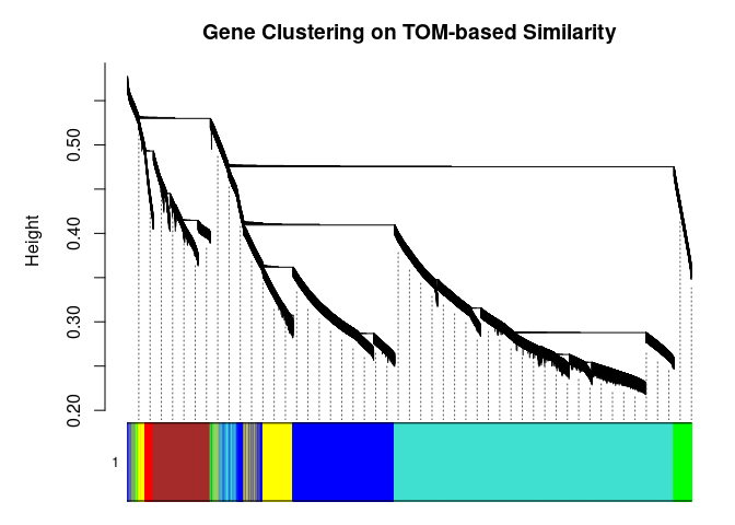
I generated a weighted adjacency matrix for the gene expression profile network using the softmax threshold I determined in the previous step. Then I generate the Topological Overlap Matrix (TOM) for the adjacency matrix. This reduces noise and spurious associations according to the authors.I use the TOM matrix to cluster the profiles of each metabolite based on their similarity. I use dynamic tree cutting to generate modules.
soft.power <- which(soft$fitIndices$SFT.R.sq >= 0.88)[1]
cat("\n", "Power chosen")
##
## Power chosensoft.power## [1] 1cat("\n \n")adj.mtx <- adjacency(log.tdata.FPKM.sample.info.subset.SM.SI.spleen.WGCNA, power=soft.power)
TOM = TOMsimilarity(adj.mtx)## ..connectivity..
## ..matrix multiplication (system BLAS)..
## ..normalization..
## ..done.diss.TOM = 1 - TOM
metabolite.clust <- hclust(as.dist(diss.TOM), method="average")
min.module.size <- 15
modules <- cutreeDynamic(dendro=metabolite.clust, distM=diss.TOM, deepSplit=2, pamRespectsDendro=FALSE, minClusterSize=min.module.size)## ..cutHeight not given, setting it to 0.574 ===> 99% of the (truncated) height range in dendro.
## ..done.# Plot modules
cols <- labels2colors(modules)
table(cols)## cols
## blue brown green red turquoise yellow
## 3960 1751 678 257 9054 1632plotDendroAndColors(
metabolite.clust, cols, xlab="", sub="", main="Gene Clustering on TOM-based Similarity",
dendroLabels=FALSE, hang=0.03, addGuide=TRUE, guideHang=0.05
)
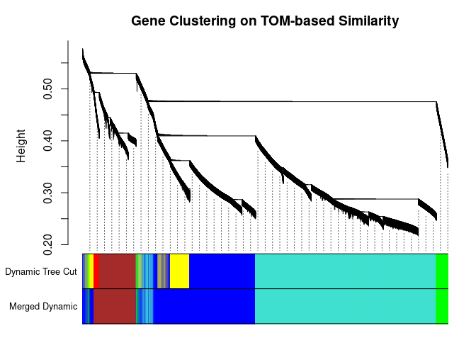
Merging Related Modules
Some modules might be highly correlated. The authors recommend merging modules with a correlation greater than 0.75.
me.list <- moduleEigengenes(log.tdata.FPKM.sample.info.subset.SM.SI.spleen.WGCNA, colors=cols)
me <- me.list$eigengenes

# Eigenmetabolite dissimilarity
me.diss <- 1 - cor(me)

h <- hclust(as.dist(me.diss), method="average")

# Merge threshold = 1 - correlation threshold
merge.thresh <- 0.25

plot(h, main="Clustering of Module Eigengene", xlab="", sub="")
abline(h=merge.thresh, col="red")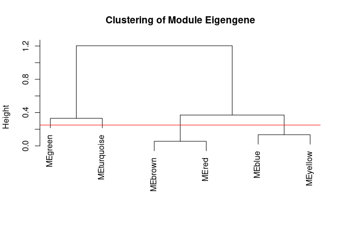
merge <- mergeCloseModules(log.tdata.FPKM.sample.info.subset.SM.SI.spleen.WGCNA, cols, cutHeight=merge.thresh, verbose=0)
merged.cols <- merge$colors
merged.mes <- merge$newMEs

  # Check how the merging changed the clustering of the metabolites
plotDendroAndColors(
  metabolite.clust, cbind(cols, merged.cols), c("Dynamic Tree Cut", "Merged Dynamic"), xlab="", sub="",
  main="Gene Clustering on TOM-based Similarity",
  dendroLabels=FALSE, hang=0.03, addGuide=TRUE, guideHang=0.05
  )
Calculating Intramodular Connectivity
This function in WGCNA calculates the total connectivity of a node (metabolite) in the network. The kTotal column specifies this connectivity. The kWithin column specifies the node connectivity within its module. The kOut column specifies the difference between kTotal and kWithin. Generally, the out degree should be lower than the within degree, since the WGCNA procedure groups similar metabolite profiles together.
net.deg <- intramodularConnectivity(adj.mtx, merged.cols)
saveRDS(net.deg,here("Data","SM.SI.spleen","Chang_2DG_BL6_connectivity_SM_SI_spleen.RData"))
head(net.deg)
## kTotal kWithin kOut kDiff
## ENSMUSG00000000001 9869.040 4196.893 5672.146 -1475.2527
## ENSMUSG00000000028 9754.058 5929.169 3824.889 2104.2803
## ENSMUSG00000000031 10374.827 4061.486 6313.341 -2251.8550
## ENSMUSG00000000037 5818.285 3575.075 2243.210 1331.8647
## ENSMUSG00000000049 3481.178 1566.518 1914.661 -348.1430
## ENSMUSG00000000056 7371.302 3359.258 4012.044 -652.7854Summary
The dataset generated coexpression modules of the following sizes. The grey submodule represents metabolites that did not fit well into any of the modules.
table(merged.cols)## merged.cols
## blue brown green turquoise
## 5592 2008 678 9054# Module names in descending order of size
module.labels <- names(table(merged.cols))[order(table(merged.cols), decreasing=T)]
# Order eigenmetabolites by module labels
merged.mes <- merged.mes[,paste0("ME", module.labels)]
colnames(merged.mes) <- paste0("log.tdata.FPKM.sample.info.subset.SM.SI.spleen.WGCNA_", module.labels)
module.eigens <- merged.mes
# Add log.tdata.FPKM.sample.info.subset.WGCNA tag to labels
module.labels <- paste0("log.tdata.FPKM.sample.info.subset.SM.SI.spleen.WGCNA_", module.labels)
# Generate and store metabolite membership
module.membership <- data.frame(
Gene=colnames(log.tdata.FPKM.sample.info.subset.SM.SI.spleen.WGCNA),
Module=paste0("log.tdata.FPKM.sample.info.subset.SM.SI.spleen.WGCNA_", merged.cols)
)
saveRDS(module.labels, here("Data","SM.SI.spleen","log.tdata.FPKM.sample.info.subset.SM.SI.spleen.WGCNA.module.labels.RData"))
saveRDS(module.eigens, here("Data","SM.SI.spleen","log.tdata.FPKM.sample.info.subset.SM.SI.spleen.WGCNA.module.eigens.RData"))
saveRDS(module.membership, here("Data","SM.SI.spleen", "log.tdata.FPKM.sample.info.subset.SM.SI.spleen.WGCNA.module.membership.RData"))
write.table(module.labels, here("Data","SM.SI.spleen","log.tdata.FPKM.sample.info.subset.SM.SI.spleen.WGCNA.module.labels.csv"), row.names=F, col.names=F, sep=",")
write.csv(module.eigens, here("Data","SM.SI.spleen","log.tdata.FPKM.sample.info.subset.SM.SI.spleen.WGCNA.module.eigens.csv"))
write.csv(module.membership, here("Data","SM.SI.spleen","log.tdata.FPKM.sample.info.subset.SM.SI.spleen.WGCNA.module.membership.csv"), row.names=F)Analysis performed by Ann Wells
The Carter Lab The Jackson Laboratory 2023
ann.wells@jax.org