Module Generation Brain
Ann Wells
April 23, 2023
log.tdata.FPKM.sample.info.subset.hip.hyp.cortex.WGCNA <- readRDS(here("Data","Brain","log.tdata.FPKM.sample.info.subset.hip.hyp.cortex.missing.WGCNA.RData"))Set Up Environment
The WGCNA package requires some strict R session environment set up.
options(stringsAsFactors=FALSE)

# Run the following only if running from terminal
# Does NOT work in RStudio
#enableWGCNAThreads()
Choosing Soft-Thresholding Power
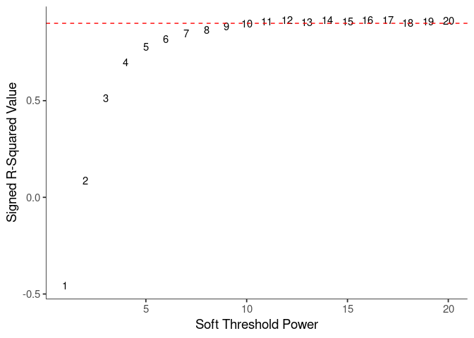
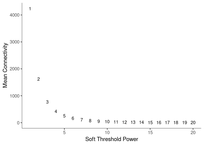
WGCNA uses a smooth softmax function to force a scale-free topology on the gene expression network. I cycled through a set of threshold power values to see which one is the best for the specific topology. As recommended by the authors, I choose the smallest power such that the scale-free topology correlation attempts to hit 0.9.
threshold <- softthreshold(soft)Scale Free Topology
Mean Connectivity
Pick Soft Threshold
knitr::kable(soft$fitIndices)| Power | SFT.R.sq | slope | truncated.R.sq | mean.k. | median.k. | max.k. |
|---|---|---|---|---|---|---|
| 1 | 0.4572816 | 1.6257692 | 0.9420347 | 4240.064348 | 4338.1167241 | 6494.4860 |
| 2 | 0.0864715 | -0.3185543 | 0.8873081 | 1623.979622 | 1614.1612335 | 3546.9323 |
| 3 | 0.5138923 | -0.9181880 | 0.9525486 | 775.694547 | 722.7128261 | 2276.1152 |
| 4 | 0.6977970 | -1.2039476 | 0.9855252 | 423.844142 | 360.3200709 | 1599.9735 |
| 5 | 0.7788052 | -1.4153573 | 0.9913897 | 253.599184 | 194.4021307 | 1196.2024 |
| 6 | 0.8193532 | -1.5522111 | 0.9898059 | 162.007936 | 111.3157232 | 930.7703 |
| 7 | 0.8491530 | -1.6338675 | 0.9900221 | 108.758234 | 66.8876899 | 745.8428 |
| 8 | 0.8644844 | -1.7052064 | 0.9870057 | 75.910541 | 41.5934621 | 611.3444 |
| 9 | 0.8822362 | -1.7424926 | 0.9876342 | 54.677783 | 26.7237722 | 510.2284 |
| 10 | 0.8974766 | -1.7672766 | 0.9891566 | 40.422334 | 17.5565030 | 432.1785 |
| 11 | 0.9092101 | -1.7814558 | 0.9896757 | 30.545811 | 11.7328587 | 370.6221 |
| 12 | 0.9159148 | -1.7930210 | 0.9908326 | 23.519325 | 8.0174652 | 321.1946 |
| 13 | 0.9045424 | -1.8185381 | 0.9792032 | 18.405750 | 5.5536692 | 280.8976 |
| 14 | 0.9150302 | -1.8062500 | 0.9829196 | 14.610416 | 3.9120138 | 247.6114 |
| 15 | 0.9106301 | -1.8182830 | 0.9773665 | 11.744555 | 2.7961644 | 219.8011 |
| 16 | 0.9179350 | -1.8102927 | 0.9795423 | 9.547338 | 2.0235262 | 196.3317 |
| 17 | 0.9162802 | -1.8127635 | 0.9785208 | 7.839746 | 1.4769222 | 176.3487 |
| 18 | 0.9007019 | -1.8309228 | 0.9656103 | 6.496410 | 1.0905098 | 159.1982 |
| 19 | 0.9078600 | -1.8174277 | 0.9684398 | 5.427941 | 0.8167131 | 144.3730 |
| 20 | 0.9123493 | -1.8088910 | 0.9707584 | 4.569566 | 0.6103708 | 131.4744 |
soft$fitIndices %>%
  download_this(
    output_name = "Soft Threshold Skeletal Muscle",
    output_extension = ".csv",
    button_label = "Download data as csv",
    button_type = "info",
    has_icon = TRUE,
    icon = "fa fa-save"
)Calculate Adjacency Matrix and Topological Overlap Matrix
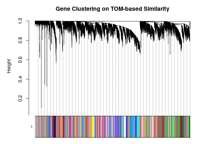
I generated a weighted adjacency matrix for the gene expression profile network using the softmax threshold I determined in the previous step. Then I generate the Topological Overlap Matrix (TOM) for the adjacency matrix. This reduces noise and spurious associations according to the authors. I use the TOM matrix to cluster the profiles of each metabolite based on their similarity. I use dynamic tree cutting to generate modules.
soft.power <- which(soft$fitIndices$SFT.R.sq >= 0.88)[1]
cat("\n", "Power chosen")
##
## Power chosensoft.power## [1] 9cat("\n \n")adj.mtx <- adjacency(log.tdata.FPKM.sample.info.subset.hip.hyp.cortex.WGCNA, power=soft.power)
TOM = TOMsimilarity(adj.mtx)## ..connectivity..
## ..matrix multiplication (system BLAS)..
## ..normalization..
## ..done.diss.TOM = 1 - TOM
metabolite.clust <- hclust(as.dist(diss.TOM), method="average")
min.module.size <- 15
modules <- cutreeDynamic(dendro=metabolite.clust, distM=diss.TOM, deepSplit=2, pamRespectsDendro=FALSE, minClusterSize=min.module.size)## ..cutHeight not given, setting it to 0.998 ===> 99% of the (truncated) height range in dendro.
## ..done.# Plot modules
cols <- labels2colors(modules)
table(cols)## cols
## aliceblue antiquewhite antiquewhite1 antiquewhite2 antiquewhite4
## 29 23 37 48 76
## bisque4 black blanchedalmond blue blue1
## 101 273 19 870 26
## blue2 blue3 blue4 blueviolet brown
## 58 32 40 40 541
## brown1 brown2 brown3 brown4 burlywood
## 32 58 26 104 18
## chocolate2 chocolate3 chocolate4 coral coral1
## 23 29 37 50 81
## coral2 coral3 coral4 cornflowerblue cornsilk
## 74 47 37 28 23
## cyan darkgoldenrod3 darkgoldenrod4 darkgreen darkgrey
## 215 19 26 178 152
## darkmagenta darkolivegreen darkolivegreen1 darkolivegreen2 darkolivegreen4
## 128 130 32 42 61
## darkorange darkorange2 darkred darkseagreen darkseagreen1
## 143 104 187 24 29
## darkseagreen2 darkseagreen3 darkseagreen4 darkslateblue darkturquoise
## 37 51 83 99 169
## darkviolet deeppink deeppink1 deeppink2 deepskyblue
## 57 40 31 26 17
## dodgerblue4 firebrick firebrick2 firebrick3 firebrick4
## 20 27 32 42 63
## floralwhite green green2 green3 green4
## 105 339 24 29 38
## greenyellow grey grey60 honeydew honeydew1
## 239 486 211 51 83
## indianred indianred1 indianred2 indianred3 indianred4
## 20 27 33 43 64
## ivory lavender lavenderblush lavenderblush1 lavenderblush2
## 107 24 30 38 53
## lavenderblush3 lightblue1 lightblue2 lightblue3 lightblue4
## 83 21 27 33 43
## lightcoral lightcyan lightcyan1 lightgreen lightpink
## 64 211 113 201 24
## lightpink1 lightpink2 lightpink3 lightpink4 lightskyblue2
## 30 38 54 85 21
## lightskyblue3 lightskyblue4 lightslateblue lightsteelblue lightsteelblue1
## 27 34 43 65 115
## lightyellow magenta magenta1 magenta2 magenta3
## 195 255 24 30 38
## magenta4 maroon mediumorchid mediumorchid3 mediumorchid4
## 54 85 74 22 27
## mediumpurple mediumpurple1 mediumpurple2 mediumpurple3 mediumpurple4
## 34 43 65 116 47
## midnightblue mistyrose mistyrose4 moccasin navajowhite
## 214 36 25 30 39
## navajowhite1 navajowhite2 navajowhite3 navajowhite4 orange
## 54 85 28 23 145
## orange3 orange4 orangered orangered1 orangered3
## 22 28 34 44 66
## orangered4 paleturquoise paleturquoise4 palevioletred palevioletred1
## 121 133 25 30 39
## palevioletred2 palevioletred3 pink pink1 pink2
## 55 90 263 22 28
## pink3 pink4 plum plum1 plum2
## 35 45 66 123 94
## plum3 plum4 powderblue purple purple2
## 57 39 31 241 25
## red red1 royalblue royalblue2 royalblue3
## 291 15 188 25 30
## saddlebrown salmon salmon1 salmon2 salmon4
## 138 218 39 55 91
## sienna sienna1 sienna2 sienna3 sienna4
## 22 28 36 126 45
## skyblue skyblue1 skyblue2 skyblue3 skyblue4
## 141 68 70 123 46
## slateblue slateblue1 slateblue2 steelblue tan
## 36 28 23 135 222
## tan2 tan3 tan4 thistle thistle1
## 25 30 39 55 93
## thistle2 thistle3 thistle4 tomato tomato2
## 94 57 39 31 25
## turquoise violet wheat3 white whitesmoke
## 1574 132 23 143 28
## yellow yellow2 yellow3 yellow4 yellowgreen
## 363 36 46 69 123plotDendroAndColors(
metabolite.clust, cols, xlab="", sub="", main="Gene Clustering on TOM-based Similarity",
dendroLabels=FALSE, hang=0.03, addGuide=TRUE, guideHang=0.05
)
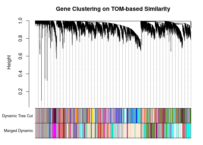
Merging Related Modules
Some modules might be highly correlated. The authors recommend merging modules with a correlation greater than 0.75.
me.list <- moduleEigengenes(log.tdata.FPKM.sample.info.subset.hip.hyp.cortex.WGCNA, colors=cols)
me <- me.list$eigengenes

# Eigenmetabolite dissimilarity
me.diss <- 1 - cor(me)

h <- hclust(as.dist(me.diss), method="average")

# Merge threshold = 1 - correlation threshold
merge.thresh <- 0.25

plot(h, main="Clustering of Module Eigengene", xlab="", sub="")
abline(h=merge.thresh, col="red")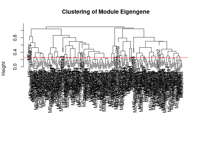
merge <- mergeCloseModules(log.tdata.FPKM.sample.info.subset.hip.hyp.cortex.WGCNA, cols, cutHeight=merge.thresh, verbose=0)
merged.cols <- merge$colors
merged.mes <- merge$newMEs

  # Check how the merging changed the clustering of the metabolites
plotDendroAndColors(
  metabolite.clust, cbind(cols, merged.cols), c("Dynamic Tree Cut", "Merged Dynamic"), xlab="", sub="",
  main="Gene Clustering on TOM-based Similarity",
  dendroLabels=FALSE, hang=0.03, addGuide=TRUE, guideHang=0.05
  )
Calculating Intramodular Connectivity
This function in WGCNA calculates the total connectivity of a node (metabolite) in the network. The kTotal column specifies this connectivity. The kWithin column specifies the node connectivity within its module. The kOut column specifies the difference between kTotal and kWithin. Generally, the out degree should be lower than the within degree, since the WGCNA procedure groups similar metabolite profiles together.
net.deg <- intramodularConnectivity(adj.mtx, merged.cols)
saveRDS(net.deg,here("Data","Brain","Chang_2DG_BL6_connectivity_hip_hyp_cortex.RData"))
head(net.deg)
## kTotal kWithin kOut kDiff
## ENSMUSG00000000001 18.58648742 5.361840218 13.22464720 -7.86280699
## ENSMUSG00000000028 0.06558317 0.004713301 0.06086987 -0.05615657
## ENSMUSG00000000031 1.47376269 0.993015063 0.48074762 0.51226744
## ENSMUSG00000000037 22.73302874 3.536517694 19.19651104 -15.65999335
## ENSMUSG00000000049 0.06781934 0.005651393 0.06216795 -0.05651655
## ENSMUSG00000000056 0.68957200 0.299373165 0.39019883 -0.09082567Summary
The dataset generated coexpression modules of the following sizes. The grey submodule represents metabolites that did not fit well into any of the modules.
table(merged.cols)## merged.cols
## aliceblue antiquewhite blanchedalmond brown1 brown3
## 62 4566 128 273 646
## burlywood chocolate3 coral3 cyan darkgrey
## 57 74 233 2192 1136
## darkolivegreen4 darkseagreen darkslateblue deeppink2 dodgerblue4
## 1280 109 353 501 20
## firebrick4 green3 green4 grey honeydew
## 339 174 155 486 300
## indianred3 lavenderblush1 lavenderblush2 lavenderblush3 lightblue1
## 66 1316 53 157 144
## lightblue2 lightcoral magenta1 magenta3 magenta4
## 27 64 425 129 343
## mediumorchid3 mediumpurple orange3 orangered1 orangered4
## 22 394 22 504 121
## paleturquoise4 pink2 plum royalblue thistle3
## 95 28 66 188 57
## wheat3
## 23# Module names in descending order of size
module.labels <- names(table(merged.cols))[order(table(merged.cols), decreasing=T)]
# Order eigenmetabolites by module labels
merged.mes <- merged.mes[,paste0("ME", module.labels)]
colnames(merged.mes) <- paste0("log.tdata.FPKM.sample.info.subset.hip.hyp.cortex.WGCNA_", module.labels)
module.eigens <- merged.mes
# Add log.tdata.FPKM.sample.info.subset.WGCNA tag to labels
module.labels <- paste0("log.tdata.FPKM.sample.info.subset.hip.hyp.cortex.WGCNA_", module.labels)
# Generate and store metabolite membership
module.membership <- data.frame(
Gene=colnames(log.tdata.FPKM.sample.info.subset.hip.hyp.cortex.WGCNA),
Module=paste0("log.tdata.FPKM.sample.info.subset.hip.hyp.cortex.WGCNA_", merged.cols)
)
saveRDS(module.labels, here("Data","Brain","log.tdata.FPKM.sample.info.subset.hip.hyp.cortex.WGCNA.module.labels.RData"))
saveRDS(module.eigens, here("Data","Brain","log.tdata.FPKM.sample.info.subset.hip.hyp.cortex.WGCNA.module.eigens.RData"))
saveRDS(module.membership, here("Data","Brain", "log.tdata.FPKM.sample.info.subset.hip.hyp.cortex.WGCNA.module.membership.RData"))
write.table(module.labels, here("Data","Brain","log.tdata.FPKM.sample.info.subset.hip.hyp.cortex.WGCNA.module.labels.csv"), row.names=F, col.names=F, sep=",")
write.csv(module.eigens, here("Data","Brain","log.tdata.FPKM.sample.info.subset.hip.hyp.cortex.WGCNA.module.eigens.csv"))
write.csv(module.membership, here("Data","Brain","log.tdata.FPKM.sample.info.subset.hip.hyp.cortex.WGCNA.module.membership.csv"), row.names=F)Analysis performed by Ann Wells
The Carter Lab The Jackson Laboratory 2023
ann.wells@jax.org