Module Generation
Ann Wells
April 23, 2023
log.tdata.FPKM.sample.info.subset.WGCNA <- readRDS(here("Data","log.tdata.FPKM.sample.info.subset.missing.WGCNA.RData"))Set Up Environment
The WGCNA package requires some strict R session environment set up.
options(stringsAsFactors=FALSE)

# Run the following only if running from terminal
# Does NOT work in RStudio
#enableWGCNAThreads()
Choosing Soft-Thresholding Power
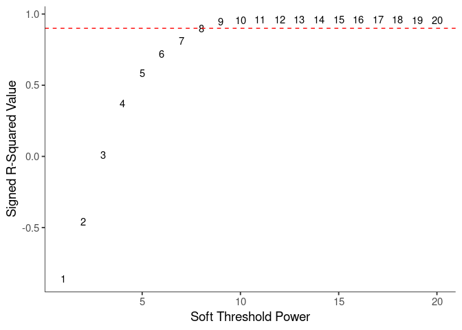
WGCNA uses a smooth softmax function to force a scale-free topology on the gene expression network. I cycled through a set of threshold power values to see which one is the best for the specific topology. As recommended by the authors, I choose the smallest power such that the scale-free topology correlation attempts to hit 0.9.
threshold <- softthreshold(soft)Scale Free Topology
Mean Connectivity
Pick Soft Threshold
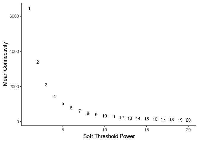
knitr::kable(soft$fitIndices)| Power | SFT.R.sq | slope | truncated.R.sq | mean.k. | median.k. | max.k. |
|---|---|---|---|---|---|---|
| 1 | 0.8612614 | 2.7655275 | 0.9878786 | 6450.08917 | 6489.58052 | 9192.6265 |
| 2 | 0.4603610 | 0.6900897 | 0.8777347 | 3403.63718 | 3317.36163 | 6173.7855 |
| 3 | 0.0115589 | -0.0654616 | 0.5811361 | 2104.88148 | 1960.49020 | 4565.3419 |
| 4 | 0.3740690 | -0.4796736 | 0.6154529 | 1428.36622 | 1261.13792 | 3615.3711 |
| 5 | 0.5856041 | -0.6794014 | 0.7173936 | 1030.57772 | 848.96741 | 2955.3740 |
| 6 | 0.7186021 | -0.7823568 | 0.8109538 | 776.74911 | 594.07548 | 2473.5780 |
| 7 | 0.8102699 | -0.8682678 | 0.8829116 | 604.94642 | 426.65977 | 2137.6500 |
| 8 | 0.8967570 | -0.9196192 | 0.9550448 | 483.36991 | 312.54528 | 1877.8028 |
| 9 | 0.9464581 | -0.9647767 | 0.9899286 | 394.28772 | 232.98209 | 1668.3541 |
| 10 | 0.9566120 | -1.0260007 | 0.9925092 | 327.16020 | 179.37372 | 1520.1972 |
| 11 | 0.9597939 | -1.0793124 | 0.9872616 | 275.39576 | 142.03410 | 1396.6941 |
| 12 | 0.9627006 | -1.1166370 | 0.9822050 | 234.69752 | 113.93864 | 1291.7740 |
| 13 | 0.9622471 | -1.1496961 | 0.9739067 | 202.16652 | 92.12115 | 1201.4449 |
| 14 | 0.9612874 | -1.1732983 | 0.9665201 | 175.78938 | 75.19930 | 1122.7884 |
| 15 | 0.9604404 | -1.1962895 | 0.9610598 | 154.13277 | 61.84509 | 1058.3629 |
| 16 | 0.9605814 | -1.2137460 | 0.9576800 | 136.15417 | 51.14912 | 1002.0938 |
| 17 | 0.9609191 | -1.2279039 | 0.9543414 | 121.08105 | 42.36921 | 951.8397 |
| 18 | 0.9607941 | -1.2413496 | 0.9517050 | 108.33143 | 35.28572 | 906.6480 |
| 19 | 0.9560648 | -1.2510075 | 0.9441395 | 97.46037 | 29.38987 | 865.7590 |
| 20 | 0.9564626 | -1.2607085 | 0.9441400 | 88.12325 | 24.88051 | 828.5598 |
soft$fitIndices %>%
  download_this(
    output_name = "Soft Threshold All Data",
    output_extension = ".csv",
    button_label = "Download data as csv",
    button_type = "info",
    has_icon = TRUE,
    icon = "fa fa-save"
)Calculate Adjacency Matrix and Topological Overlap Matrix
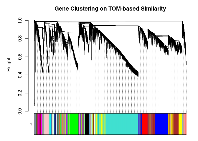
I generated a weighted adjacency matrix for the gene expression profile network using the softmax threshold I determined in the previous step. Then I generate the Topological Overlap Matrix (TOM) for the adjacency matrix. This reduces noise and spurious associations according to the authors. I use the TOM matrix to cluster the profiles of each metabolite based on their similarity. I use dynamic tree cutting to generate modules.
soft.power <- 8
cat("\n", "Power chosen")
##
## Power chosensoft.power## [1] 8cat("\n \n")adj.mtx <- adjacency(log.tdata.FPKM.sample.info.subset.WGCNA, power=soft.power)
TOM = TOMsimilarity(adj.mtx)## ..connectivity..
## ..matrix multiplication (system BLAS)..
## ..normalization..
## ..done.diss.TOM = 1 - TOM
metabolite.clust <- hclust(as.dist(diss.TOM), method="average")
min.module.size <- 15
modules <- cutreeDynamic(dendro=metabolite.clust, distM=diss.TOM, deepSplit=2, pamRespectsDendro=FALSE, minClusterSize=min.module.size)## ..cutHeight not given, setting it to 0.995 ===> 99% of the (truncated) height range in dendro.
## ..done.# Plot modules
cols <- labels2colors(modules)
table(cols)## cols
## black blue brown brown4 cyan
## 500 1798 1634 30 231
## darkgreen darkgrey darkmagenta darkolivegreen darkorange
## 134 127 85 86 113
## darkorange2 darkred darkturquoise floralwhite green
## 38 158 128 40 1214
## greenyellow grey grey60 ivory lightcyan
## 404 29 198 44 210
## lightcyan1 lightgreen lightsteelblue1 lightyellow magenta
## 45 175 56 169 450
## mediumpurple3 midnightblue orange orangered4 paleturquoise
## 57 228 117 58 93
## pink plum1 purple red royalblue
## 487 62 445 665 165
## saddlebrown salmon sienna3 skyblue skyblue3
## 100 254 82 103 65
## steelblue tan turquoise violet white
## 96 326 4287 87 108
## yellow yellowgreen
## 1274 77plotDendroAndColors(
metabolite.clust, cols, xlab="", sub="", main="Gene Clustering on TOM-based Similarity",
dendroLabels=FALSE, hang=0.03, addGuide=TRUE, guideHang=0.05
)
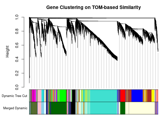
Merging Related Modules
Some modules might be highly correlated. The authors recommend merging modules with a correlation greater than 0.75.
me.list <- moduleEigengenes(log.tdata.FPKM.sample.info.subset.WGCNA, colors=cols)
me <- me.list$eigengenes

# Eigenmetabolite dissimilarity
me.diss <- 1 - cor(me)

h <- hclust(as.dist(me.diss), method="average")

# Merge threshold = 1 - correlation threshold
merge.thresh <- 0.25

plot(h, main="Clustering of Module Eigengene", xlab="", sub="")
abline(h=merge.thresh, col="red")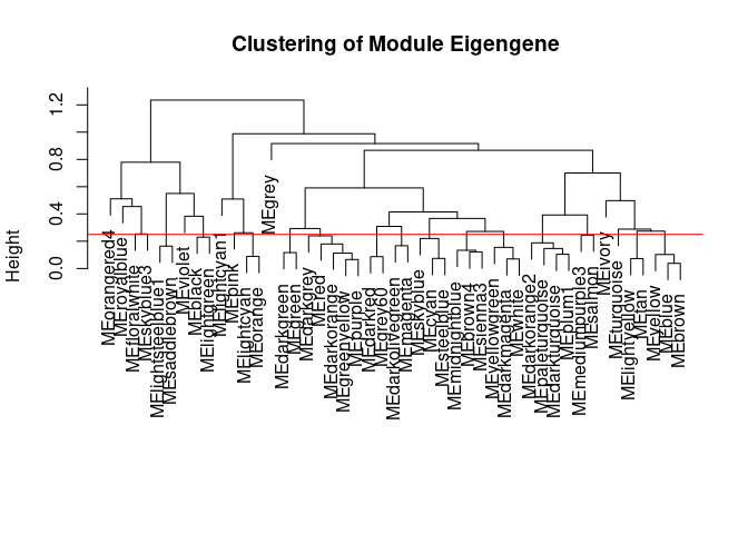
merge <- mergeCloseModules(log.tdata.FPKM.sample.info.subset.WGCNA, cols, cutHeight=merge.thresh, verbose=0)
merged.cols <- merge$colors
merged.mes <- merge$newMEs

  # Check how the merging changed the clustering of the metabolites
plotDendroAndColors(
  metabolite.clust, cbind(cols, merged.cols), c("Dynamic Tree Cut", "Merged Dynamic"), xlab="", sub="",
  main="Gene Clustering on TOM-based Similarity",
  dendroLabels=FALSE, hang=0.03, addGuide=TRUE, guideHang=0.05
  )
Calculating Intramodular Connectivity
This function in WGCNA calculates the total connectivity of a node (metabolite) in the network. The kTotal column specifies this connectivity. The kWithin column specifies the node connectivity within its module. The kOut column specifies the difference between kTotal and kWithin. Generally, the out degree should be lower than the within degree, since the WGCNA procedure groups similar metabolite profiles together.
net.deg <- intramodularConnectivity(adj.mtx, merged.cols)
saveRDS(net.deg,here("Data","Chang_2DG_BL6_connectivity.RData"))
head(net.deg)
## kTotal kWithin kOut kDiff
## ENSMUSG00000000001 296.99507 99.48080 197.51426 -98.03346441
## ENSMUSG00000000028 376.29779 343.86570 32.43209 311.43360697
## ENSMUSG00000000031 216.08673 116.59827 99.48846 17.10980402
## ENSMUSG00000000037 142.45133 73.60603 68.84530 4.76072455
## ENSMUSG00000000049 241.81391 115.13560 126.67831 -11.54270168
## ENSMUSG00000000056 56.11815 28.09418 28.02397 0.07020203Summary
The dataset generated coexpression modules of the following sizes. The grey submodule represents metabolites that did not fit well into any of the modules.
table(merged.cols)## merged.cols
## black darkgreen darkolivegreen darkorange2 floralwhite
## 675 3102 892 321 40
## grey ivory lightcyan lightcyan1 lightsteelblue1
## 29 44 327 45 156
## lightyellow mediumpurple3 midnightblue orangered4 pink
## 5201 311 610 58 487
## royalblue skyblue skyblue3 turquoise violet
## 165 430 65 4287 87# Module names in descending order of size
module.labels <- names(table(merged.cols))[order(table(merged.cols), decreasing=T)]
# Order eigenmetabolites by module labels
merged.mes <- merged.mes[,paste0("ME", module.labels)]
colnames(merged.mes) <- paste0("log.tdata.FPKM.sample.info.subset.WGCNA_", module.labels)
module.eigens <- merged.mes
# Add log.tdata.FPKM.sample.info.subset.WGCNA tag to labels
module.labels <- paste0("log.tdata.FPKM.sample.info.subset.WGCNA_", module.labels)
# Generate and store metabolite membership
module.membership <- data.frame(
Gene=colnames(log.tdata.FPKM.sample.info.subset.WGCNA),
Module=paste0("log.tdata.FPKM.sample.info.subset.WGCNA_", merged.cols)
)
saveRDS(module.labels, here("Data","log.tdata.FPKM.sample.info.subset.WGCNA.module.labels.RData"))
saveRDS(module.eigens, here("Data","log.tdata.FPKM.sample.info.subset.WGCNA.module.eigens.RData"))
saveRDS(module.membership, here("Data", "log.tdata.FPKM.sample.info.subset.WGCNA.module.membership.RData"))
write.table(module.labels, here("Data","log.tdata.FPKM.sample.info.subset.WGCNA.module.labels.csv"), row.names=F, col.names=F, sep=",")
write.csv(module.eigens, here("Data","log.tdata.FPKM.sample.info.subset.WGCNA.module.eigens.csv"))
write.csv(module.membership, here("Data","log.tdata.FPKM.sample.info.subset.WGCNA.module.membership.csv"), row.names=F)Analysis performed by Ann Wells
The Carter Lab The Jackson Laboratory 2023
ann.wells@jax.org