Module Generation Hippocampus
Ann Wells
April 23, 2023
log.tdata.FPKM.sample.info.subset.hippocampus.WGCNA <- readRDS(here("Data","Hippocampus","log.tdata.FPKM.sample.info.subset.hippocampus.missing.WGCNA.RData"))Set Up Environment
The WGCNA package requires some strict R session environment set up.
options(stringsAsFactors=FALSE)

# Run the following only if running from terminal
# Does NOT work in RStudio
#enableWGCNAThreads()
Choosing Soft-Thresholding Power
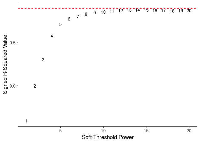
WGCNA uses a smooth softmax function to force a scale-free topology on the gene expression network. I cycled through a set of threshold power values to see which one is the best for the specific topology. As recommended by the authors, I choose the smallest power such that the scale-free topology correlation attempts to hit 0.9.
threshold <- softthreshold(soft)Scale Free Topology
Mean Connectivity
Pick Soft Threshold
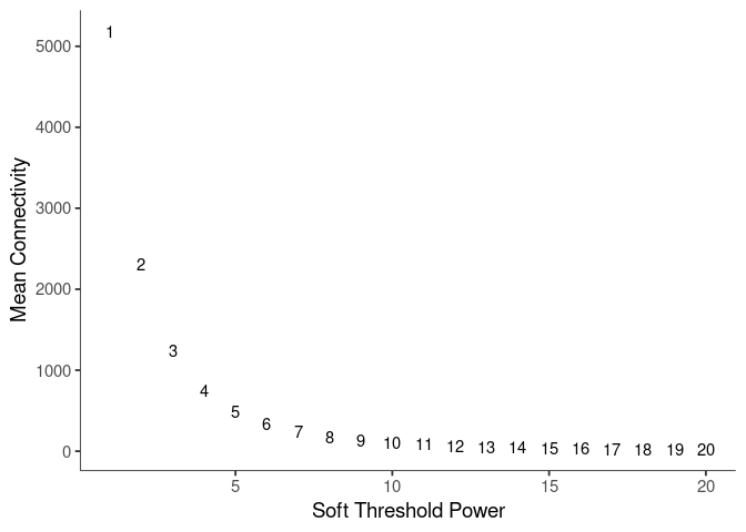
knitr::kable(soft$fitIndices)| Power | SFT.R.sq | slope | truncated.R.sq | mean.k. | median.k. | max.k. |
|---|---|---|---|---|---|---|
| 1 | 0.4079964 | 2.0927562 | 0.9760045 | 5186.30383 | 5169.731435 | 7489.8793 |
| 2 | 0.0003620 | 0.0252823 | 0.9402281 | 2309.97330 | 2221.124114 | 4452.6152 |
| 3 | 0.3048512 | -0.6485164 | 0.9369338 | 1242.70364 | 1134.543627 | 3027.8194 |
| 4 | 0.5805026 | -0.9863425 | 0.9430913 | 749.24279 | 646.246990 | 2219.8929 |
| 5 | 0.7156176 | -1.1752284 | 0.9575467 | 487.84318 | 394.159707 | 1706.1384 |
| 6 | 0.7784009 | -1.3073241 | 0.9629305 | 335.78818 | 253.009023 | 1361.2810 |
| 7 | 0.8068460 | -1.3969717 | 0.9642598 | 241.05554 | 168.847633 | 1114.2592 |
| 8 | 0.8336637 | -1.4642735 | 0.9703181 | 178.85087 | 116.463865 | 929.7016 |
| 9 | 0.8509590 | -1.5011963 | 0.9757570 | 136.27174 | 82.656137 | 787.6522 |
| 10 | 0.8570546 | -1.5326233 | 0.9772658 | 106.12726 | 59.646699 | 675.6949 |
| 11 | 0.8694827 | -1.5553759 | 0.9824845 | 84.18251 | 43.965390 | 585.7250 |
| 12 | 0.8747122 | -1.5780730 | 0.9832371 | 67.82768 | 32.932464 | 512.2439 |
| 13 | 0.8814833 | -1.6004352 | 0.9854642 | 55.39230 | 24.968371 | 451.4001 |
| 14 | 0.8817532 | -1.6182802 | 0.9856113 | 45.77205 | 19.249342 | 401.7164 |
| 15 | 0.8806436 | -1.6364880 | 0.9848720 | 38.21639 | 15.025989 | 359.7430 |
| 16 | 0.8729426 | -1.6636303 | 0.9807670 | 32.20277 | 11.811475 | 323.8298 |
| 17 | 0.8765087 | -1.6729422 | 0.9834147 | 27.35958 | 9.353385 | 292.8517 |
| 18 | 0.8721744 | -1.6892395 | 0.9809100 | 23.41761 | 7.507886 | 265.9375 |
| 19 | 0.8747841 | -1.6965775 | 0.9819909 | 20.17850 | 6.049741 | 242.4029 |
| 20 | 0.8758682 | -1.7044245 | 0.9835190 | 17.49392 | 4.906542 | 221.7041 |
soft$fitIndices %>%
  download_this(
    output_name = "Soft Threshold Hippocampus",
    output_extension = ".csv",
    button_label = "Download data as csv",
    button_type = "info",
    has_icon = TRUE,
    icon = "fa fa-save"
)Calculate Adjacency Matrix and Topological Overlap Matrix
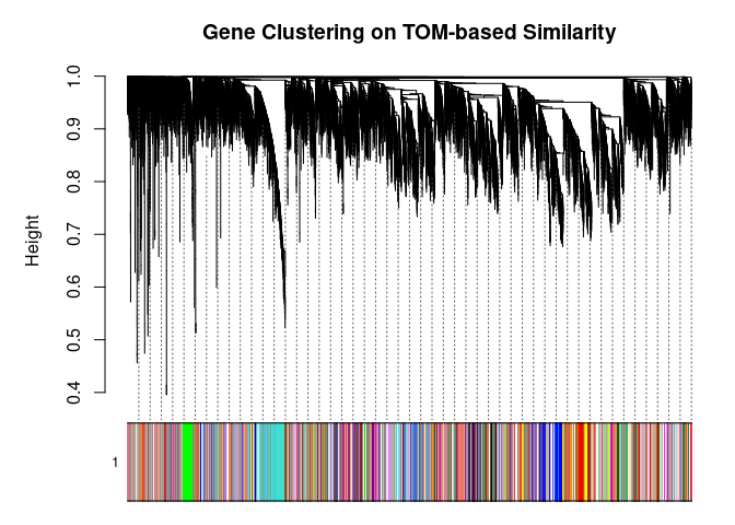
I generated a weighted adjacency matrix for the gene expression profile network using the softmax threshold I determined in the previous step. Then I generate the Topological Overlap Matrix (TOM) for the adjacency matrix. This reduces noise and spurious associations according to the authors.I use the TOM matrix to cluster the profiles of each metabolite based on their similarity. I use dynamic tree cutting to generate modules.
soft.power <- which(soft$fitIndices$SFT.R.sq >= 0.88)[1]
cat("\n", "Power chosen")
##
## Power chosensoft.power## [1] 13cat("\n \n")adj.mtx <- adjacency(log.tdata.FPKM.sample.info.subset.hippocampus.WGCNA, power=soft.power)
TOM = TOMsimilarity(adj.mtx)## ..connectivity..
## ..matrix multiplication (system BLAS)..
## ..normalization..
## ..done.diss.TOM = 1 - TOM
metabolite.clust <- hclust(as.dist(diss.TOM), method="average")
min.module.size <- 15
modules <- cutreeDynamic(dendro=metabolite.clust, distM=diss.TOM, deepSplit=2, pamRespectsDendro=FALSE, minClusterSize=min.module.size)## ..cutHeight not given, setting it to 0.998 ===> 99% of the (truncated) height range in dendro.
## ..done.# Plot modules
cols <- labels2colors(modules)
table(cols)## cols
## aliceblue antiquewhite antiquewhite1
## 45 37 51
## antiquewhite2 antiquewhite3 antiquewhite4
## 59 32 72
## aquamarine bisque2 bisque3
## 24 19 28
## bisque4 black blanchedalmond
## 82 232 35
## blue blue1 blue2
## 534 41 66
## blue3 blue4 blueviolet
## 48 54 55
## brown brown1 brown2
## 380 48 66
## brown3 brown4 burlywood
## 40 83 35
## burlywood1 chocolate chocolate1
## 28 25 33
## chocolate2 chocolate3 chocolate4
## 38 45 51
## coral coral1 coral2
## 59 72 71
## coral3 coral4 cornflowerblue
## 59 51 44
## cornsilk cornsilk2 cyan
## 37 32 172
## cyan1 darkgoldenrod darkgoldenrod1
## 24 20 28
## darkgoldenrod3 darkgoldenrod4 darkgreen
## 35 41 117
## darkgrey darkmagenta darkolivegreen
## 113 91 92
## darkolivegreen1 darkolivegreen2 darkolivegreen4
## 48 55 67
## darkorange darkorange2 darkorchid4
## 110 83 25
## darkred darksalmon darkseagreen
## 119 33 38
## darkseagreen1 darkseagreen2 darkseagreen3
## 45 51 60
## darkseagreen4 darkslateblue darkturquoise
## 72 82 116
## darkviolet deeppink deeppink1
## 65 54 48
## deeppink2 deepskyblue deepskyblue4
## 40 34 28
## dodgerblue1 dodgerblue3 dodgerblue4
## 20 29 35
## firebrick firebrick2 firebrick3
## 41 48 55
## firebrick4 floralwhite goldenrod4
## 68 84 25
## green green1 green2
## 299 33 38
## green3 green4 greenyellow
## 46 51 198
## grey grey60 honeydew
## 269 142 61
## honeydew1 hotpink3 hotpink4
## 73 20 29
## indianred indianred1 indianred2
## 36 41 48
## indianred3 indianred4 ivory
## 56 68 84
## khaki3 khaki4 lavender
## 25 33 38
## lavenderblush lavenderblush1 lavenderblush2
## 46 51 62
## lavenderblush3 lemonchiffon4 lightblue
## 74 21 29
## lightblue1 lightblue2 lightblue3
## 36 41 49
## lightblue4 lightcoral lightcyan
## 56 68 147
## lightcyan1 lightgoldenrod4 lightgoldenrodyellow
## 85 25 33
## lightgreen lightpink lightpink1
## 134 38 46
## lightpink2 lightpink3 lightpink4
## 52 62 75
## lightskyblue lightskyblue1 lightskyblue2
## 21 30 36
## lightskyblue3 lightskyblue4 lightslateblue
## 41 49 56
## lightsteelblue lightsteelblue1 lightyellow
## 68 85 126
## limegreen linen magenta
## 26 33 222
## magenta1 magenta2 magenta3
## 38 46 52
## magenta4 maroon mediumorchid
## 62 76 71
## mediumorchid1 mediumorchid2 mediumorchid3
## 22 30 36
## mediumorchid4 mediumpurple mediumpurple1
## 42 49 57
## mediumpurple2 mediumpurple3 mediumpurple4
## 69 86 58
## midnightblue mistyrose mistyrose2
## 170 51 26
## mistyrose3 mistyrose4 moccasin
## 34 39 46
## navajowhite navajowhite1 navajowhite2
## 53 63 76
## navajowhite3 navajowhite4 oldlace
## 44 37 32
## olivedrab4 orange orange1
## 22 112 24
## orange2 orange3 orange4
## 30 36 42
## orangered orangered1 orangered3
## 50 57 69
## orangered4 paleturquoise paleturquoise1
## 87 97 27
## paleturquoise3 paleturquoise4 palevioletred
## 34 39 46
## palevioletred1 palevioletred2 palevioletred3
## 53 63 78
## peachpuff4 peru pink
## 22 31 231
## pink1 pink2 pink3
## 37 43 50
## pink4 plum plum1
## 58 69 89
## plum2 plum3 plum4
## 81 65 54
## powderblue purple purple2
## 48 216 40
## red red1 red4
## 257 34 27
## rosybrown3 rosybrown4 royalblue
## 27 34 125
## royalblue2 royalblue3 saddlebrown
## 39 47 98
## salmon salmon1 salmon2
## 182 53 63
## salmon4 seashell3 seashell4
## 79 23 31
## sienna sienna1 sienna2
## 37 43 50
## sienna3 sienna4 skyblue
## 91 58 103
## skyblue1 skyblue2 skyblue3
## 70 70 89
## skyblue4 slateblue slateblue1
## 58 51 44
## slateblue2 slateblue3 slateblue4
## 37 32 24
## steelblue steelblue4 tan
## 98 27 183
## tan1 tan2 tan3
## 34 39 47
## tan4 thistle thistle1
## 53 63 80
## thistle2 thistle3 thistle4
## 81 64 53
## tomato tomato2 tomato4
## 47 39 34
## turquoise turquoise2 violet
## 899 27 94
## violetred4 wheat1 wheat3
## 23 31 37
## white whitesmoke yellow
## 109 44 367
## yellow2 yellow3 yellow4
## 50 58 70
## yellowgreen
## 90plotDendroAndColors(
metabolite.clust, cols, xlab="", sub="", main="Gene Clustering on TOM-based Similarity",
dendroLabels=FALSE, hang=0.03, addGuide=TRUE, guideHang=0.05
)
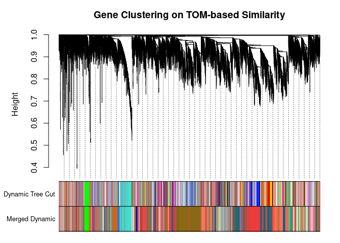
Merging Related Modules
Some modules might be highly correlated. The authors recommend merging modules with a correlation greater than 0.75.
me.list <- moduleEigengenes(log.tdata.FPKM.sample.info.subset.hippocampus.WGCNA, colors=cols)
me <- me.list$eigengenes

# Eigenmetabolite dissimilarity
me.diss <- 1 - cor(me)

h <- hclust(as.dist(me.diss), method="average")

# Merge threshold = 1 - correlation threshold
merge.thresh <- 0.25

plot(h, main="Clustering of Module Eigengene", xlab="", sub="")
abline(h=merge.thresh, col="red")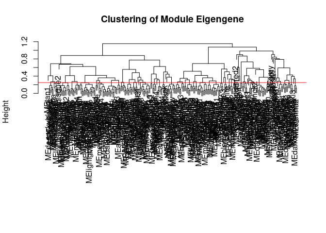
merge <- mergeCloseModules(log.tdata.FPKM.sample.info.subset.hippocampus.WGCNA, cols, cutHeight=merge.thresh, verbose=0)
merged.cols <- merge$colors
merged.mes <- merge$newMEs

  # Check how the merging changed the clustering of the metabolites
plotDendroAndColors(
  metabolite.clust, cbind(cols, merged.cols), c("Dynamic Tree Cut", "Merged Dynamic"), xlab="", sub="",
  main="Gene Clustering on TOM-based Similarity",
  dendroLabels=FALSE, hang=0.03, addGuide=TRUE, guideHang=0.05
  )
Calculating Intramodular Connectivity
This function in WGCNA calculates the total connectivity of a node (metabolite) in the network. The kTotal column specifies this connectivity. The kWithin column specifies the node connectivity within its module. The kOut column specifies the difference between kTotal and kWithin. Generally, the out degree should be lower than the within degree, since the WGCNA procedure groups similar metabolite profiles together.
net.deg <- intramodularConnectivity(adj.mtx, merged.cols)
saveRDS(net.deg,here("Data","Hippocampus","Chang_2DG_BL6_connectivity_hippocampus.RData"))
head(net.deg)
## kTotal kWithin kOut kDiff
## ENSMUSG00000000001 41.166373 21.6199608 19.546412 2.0735484
## ENSMUSG00000000028 1.942298 0.4153271 1.526971 -1.1116438
## ENSMUSG00000000031 1.361926 0.1374476 1.224478 -1.0870307
## ENSMUSG00000000037 1.971387 0.5277179 1.443670 -0.9159517
## ENSMUSG00000000049 1.302443 0.1945063 1.107936 -0.9134301
## ENSMUSG00000000056 3.542715 2.2634399 1.279275 0.9841645Summary
The dataset generated coexpression modules of the following sizes. The grey submodule represents metabolites that did not fit well into any of the modules.
table(merged.cols)## merged.cols
## antiquewhite bisque2 blanchedalmond blue1 blue3
## 37 19 128 41 129
## brown1 brown2 chocolate chocolate2 chocolate3
## 568 2163 57 75 792
## coral1 darkgoldenrod1 darkgoldenrod4 darkgrey darkolivegreen
## 1683 28 41 721 123
## darkseagreen2 darkslateblue deeppink deepskyblue4 dodgerblue1
## 807 295 54 1909 380
## dodgerblue3 firebrick2 firebrick3 goldenrod4 green
## 82 48 55 2769 299
## green3 grey indianred1 indianred2 indianred4
## 90 269 452 48 232
## khaki3 lavenderblush1 lavenderblush2 lavenderblush3 orange3
## 25 51 265 74 36
## orangered1 pink1 pink4 rosybrown3 salmon1
## 57 543 149 27 53
## slateblue1 tan1 tan4 tomato turquoise
## 142 34 414 152 899# Module names in descending order of size
module.labels <- names(table(merged.cols))[order(table(merged.cols), decreasing=T)]
# Order eigenmetabolites by module labels
merged.mes <- merged.mes[,paste0("ME", module.labels)]
colnames(merged.mes) <- paste0("log.tdata.FPKM.sample.info.subset.hippocampus.WGCNA_", module.labels)
module.eigens <- merged.mes
# Add log.tdata.FPKM.sample.info.subset.WGCNA tag to labels
module.labels <- paste0("log.tdata.FPKM.sample.info.subset.hippocampus.WGCNA_", module.labels)
# Generate and store metabolite membership
module.membership <- data.frame(
Gene=colnames(log.tdata.FPKM.sample.info.subset.hippocampus.WGCNA),
Module=paste0("log.tdata.FPKM.sample.info.subset.hippocampus.WGCNA_", merged.cols)
)
saveRDS(module.labels, here("Data","Hippocampus","log.tdata.FPKM.sample.info.subset.hippocampus.WGCNA.module.labels.RData"))
saveRDS(module.eigens, here("Data","Hippocampus","log.tdata.FPKM.sample.info.subset.hippocampus.WGCNA.module.eigens.RData"))
saveRDS(module.membership, here("Data","Hippocampus", "log.tdata.FPKM.sample.info.subset.hippocampus.WGCNA.module.membership.RData"))
write.table(module.labels, here("Data","Hippocampus","log.tdata.FPKM.sample.info.subset.hippocampus.WGCNA.module.labels.csv"), row.names=F, col.names=F, sep=",")
write.csv(module.eigens, here("Data","Hippocampus","log.tdata.FPKM.sample.info.subset.hippocampus.WGCNA.module.eigens.csv"))
write.csv(module.membership, here("Data","Hippocampus","log.tdata.FPKM.sample.info.subset.hippocampus.WGCNA.module.membership.csv"), row.names=F)Analysis performed by Ann Wells
The Carter Lab The Jackson Laboratory 2023
ann.wells@jax.org