Module Generation Skeletal Muscle
Ann Wells
April 23, 2023
log.tdata.FPKM.sample.info.subset.skeletal.muscle.WGCNA <- readRDS(here("Data","Skeletal Muscle","log.tdata.FPKM.sample.info.subset.skeletal.muscle.missing.WGCNA.RData"))Set Up Environment
The WGCNA package requires some strict R session environment set up.
options(stringsAsFactors=FALSE)

# Run the following only if running from terminal
# Does NOT work in RStudio
#enableWGCNAThreads()
Choosing Soft-Thresholding Power
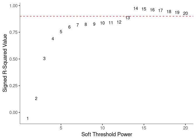
WGCNA uses a smooth softmax function to force a scale-free topology on the gene expression network. I cycled through a set of threshold power values to see which one is the best for the specific topology. As recommended by the authors, I choose the smallest power such that the scale-free topology correlation attempts to hit 0.9.
threshold <- softthreshold(soft)Scale Free Topology
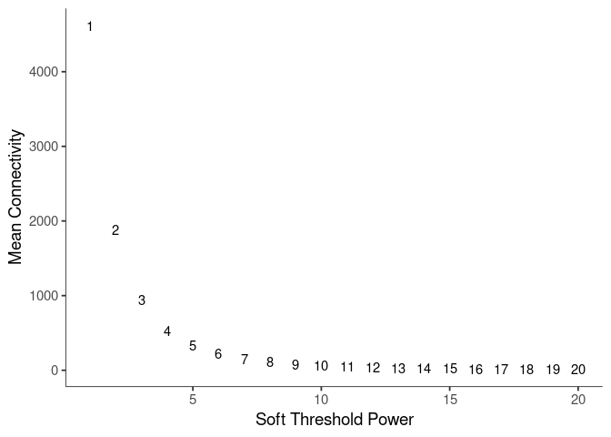
Mean Connectivity
Pick Soft Threshold
knitr::kable(soft$fitIndices)| Power | SFT.R.sq | slope | truncated.R.sq | mean.k. | median.k. | max.k. |
|---|---|---|---|---|---|---|
| 1 | 0.0558023 | 0.8376776 | 0.8325746 | 4617.01805 | 4626.320037 | 6609.3377 |
| 2 | 0.1296802 | -0.6666806 | 0.8746160 | 1878.53629 | 1809.240446 | 3600.8574 |
| 3 | 0.5033308 | -1.1517859 | 0.9479098 | 938.61962 | 845.471372 | 2280.9094 |
| 4 | 0.6910738 | -1.4537832 | 0.9604109 | 532.56173 | 457.259124 | 1599.8666 |
| 5 | 0.7561457 | -1.5836908 | 0.9635950 | 329.79400 | 263.484093 | 1190.0917 |
| 6 | 0.7987305 | -1.6607498 | 0.9699628 | 217.78960 | 161.985906 | 921.9063 |
| 7 | 0.8194878 | -1.7004239 | 0.9705365 | 151.12185 | 105.715869 | 735.7267 |
| 8 | 0.8248882 | -1.7399253 | 0.9667007 | 109.08270 | 70.956185 | 600.6698 |
| 9 | 0.8273789 | -1.7551649 | 0.9613244 | 81.32576 | 48.459887 | 499.3066 |
| 10 | 0.8369717 | -1.7445705 | 0.9582433 | 62.29640 | 34.213487 | 421.1387 |
| 11 | 0.8391725 | -1.7213139 | 0.9438019 | 48.83445 | 24.603272 | 359.9479 |
| 12 | 0.8471460 | -1.6830544 | 0.9262043 | 39.05403 | 18.179647 | 311.4112 |
| 13 | 0.8870833 | -1.5907207 | 0.9273653 | 31.78355 | 13.579538 | 271.8521 |
| 14 | 0.9750857 | -1.4730409 | 0.9859834 | 26.26989 | 10.299625 | 239.1669 |
| 15 | 0.9696071 | -1.5241373 | 0.9781512 | 22.01441 | 7.902834 | 231.0463 |
| 16 | 0.9611069 | -1.5623170 | 0.9648310 | 18.67832 | 6.135861 | 224.1249 |
| 17 | 0.9553664 | -1.5865117 | 0.9525216 | 16.02621 | 4.805901 | 217.7961 |
| 18 | 0.9433595 | -1.6034592 | 0.9339225 | 13.89111 | 3.802684 | 211.9707 |
| 19 | 0.9354704 | -1.6052041 | 0.9199804 | 12.15251 | 3.031077 | 206.5781 |
| 20 | 0.9286027 | -1.5977471 | 0.9087223 | 10.72195 | 2.439770 | 201.5618 |
soft$fitIndices %>%
  download_this(
    output_name = "Soft Threshold Skeletal Muscle",
    output_extension = ".csv",
    button_label = "Download data as csv",
    button_type = "info",
    has_icon = TRUE,
    icon = "fa fa-save"
)Calculate Adjacency Matrix and Topological Overlap Matrix
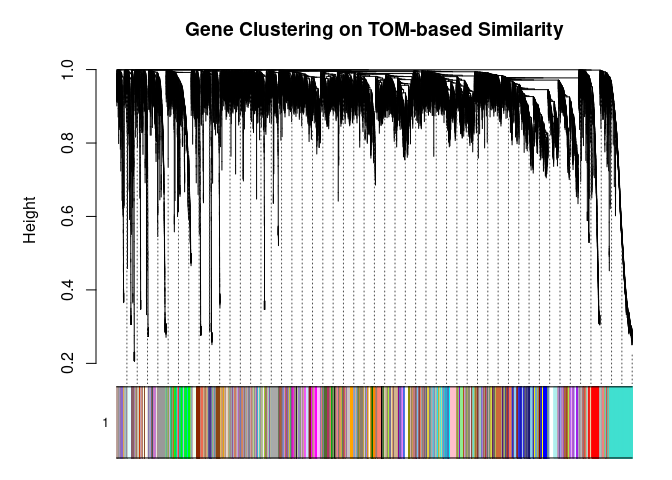
I generated a weighted adjacency matrix for the gene expression profile network using the softmax threshold I determined in the previous step. Then I generate the Topological Overlap Matrix (TOM) for the adjacency matrix. This reduces noise and spurious associations according to the authors.I use the TOM matrix to cluster the profiles of each metabolite based on their similarity. I use dynamic tree cutting to generate modules.
soft.power <- which(soft$fitIndices$SFT.R.sq >= 0.88)[1]
cat("\n", "Power chosen")
##
## Power chosensoft.power## [1] 13cat("\n \n")adj.mtx <- adjacency(log.tdata.FPKM.sample.info.subset.skeletal.muscle.WGCNA, power=soft.power)
TOM = TOMsimilarity(adj.mtx)## ..connectivity..
## ..matrix multiplication (system BLAS)..
## ..normalization..
## ..done.diss.TOM = 1 - TOM
metabolite.clust <- hclust(as.dist(diss.TOM), method="average")
min.module.size <- 15
modules <- cutreeDynamic(dendro=metabolite.clust, distM=diss.TOM, deepSplit=2, pamRespectsDendro=FALSE, minClusterSize=min.module.size)## ..cutHeight not given, setting it to 0.996 ===> 99% of the (truncated) height range in dendro.
## ..done.# Plot modules
cols <- labels2colors(modules)
table(cols)## cols
## antiquewhite2 antiquewhite4 bisque4 black blue
## 38 102 127 385 586
## blue2 brown brown2 brown4 coral
## 63 546 76 134 40
## coral1 coral2 coral3 cyan darkgreen
## 103 98 38 319 260
## darkgrey darkmagenta darkolivegreen darkolivegreen4 darkorange
## 229 181 186 80 217
## darkorange2 darkred darkseagreen3 darkseagreen4 darkslateblue
## 136 262 43 106 121
## darkturquoise darkviolet firebrick4 floralwhite green
## 243 63 82 143 467
## greenyellow grey grey60 honeydew honeydew1
## 326 453 300 43 106
## indianred4 ivory lavenderblush2 lavenderblush3 lightcoral
## 85 145 44 109 85
## lightcyan lightcyan1 lightgreen lightpink3 lightpink4
## 305 152 298 46 112
## lightsteelblue lightsteelblue1 lightyellow magenta magenta4
## 85 154 296 339 50
## maroon mediumorchid mediumpurple2 mediumpurple3 mediumpurple4
## 113 98 87 154 37
## midnightblue navajowhite1 navajowhite2 orange orangered1
## 312 50 117 224 28
## orangered3 orangered4 paleturquoise palevioletred2 palevioletred3
## 89 162 201 52 119
## pink pink4 plum plum1 plum2
## 380 29 91 167 121
## plum3 purple red royalblue saddlebrown
## 60 338 407 277 204
## salmon salmon2 salmon4 sienna3 sienna4
## 322 55 120 179 29
## skyblue skyblue1 skyblue2 skyblue3 skyblue4
## 207 92 98 171 36
## steelblue tan thistle thistle1 thistle2
## 204 323 57 120 121
## thistle3 turquoise violet white yellow
## 58 893 199 208 487
## yellow3 yellow4 yellowgreen
## 36 93 178plotDendroAndColors(
metabolite.clust, cols, xlab="", sub="", main="Gene Clustering on TOM-based Similarity",
dendroLabels=FALSE, hang=0.03, addGuide=TRUE, guideHang=0.05
)
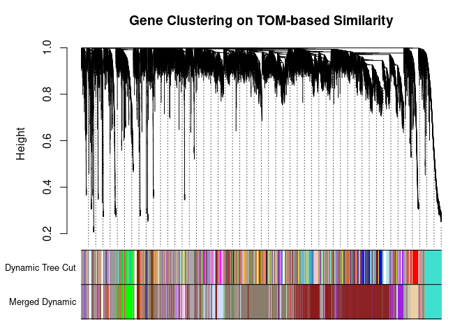
Merging Related Modules
Some modules might be highly correlated. The authors recommend merging modules with a correlation greater than 0.75.
me.list <- moduleEigengenes(log.tdata.FPKM.sample.info.subset.skeletal.muscle.WGCNA, colors=cols)
me <- me.list$eigengenes

# Eigenmetabolite dissimilarity
me.diss <- 1 - cor(me)

h <- hclust(as.dist(me.diss), method="average")

# Merge threshold = 1 - correlation threshold
merge.thresh <- 0.25

plot(h, main="Clustering of Module Eigengene", xlab="", sub="")
abline(h=merge.thresh, col="red")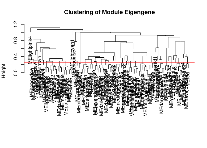
merge <- mergeCloseModules(log.tdata.FPKM.sample.info.subset.skeletal.muscle.WGCNA, cols, cutHeight=merge.thresh, verbose=0)
merged.cols <- merge$colors
merged.mes <- merge$newMEs

  # Check how the merging changed the clustering of the metabolites
plotDendroAndColors(
  metabolite.clust, cbind(cols, merged.cols), c("Dynamic Tree Cut", "Merged Dynamic"), xlab="", sub="",
  main="Gene Clustering on TOM-based Similarity",
  dendroLabels=FALSE, hang=0.03, addGuide=TRUE, guideHang=0.05
  )
Calculating Intramodular Connectivity
This function in WGCNA calculates the total connectivity of a node (metabolite) in the network. The kTotal column specifies this connectivity. The kWithin column specifies the node connectivity within its module. The kOut column specifies the difference between kTotal and kWithin. Generally, the out degree should be lower than the within degree, since the WGCNA procedure groups similar metabolite profiles together.
net.deg <- intramodularConnectivity(adj.mtx, merged.cols)
saveRDS(net.deg,here("Data","Skeletal Muscle","Chang_2DG_BL6_connectivity_muscle.RData"))

head(net.deg)
## kTotal kWithin kOut kDiff
## ENSMUSG00000000001 23.7940352 14.04376351 9.7502717 4.2934918
## ENSMUSG00000000028 1.0721016 0.08170898 0.9903926 -0.9086836
## ENSMUSG00000000031 29.9734883 25.45557442 4.5179139 20.9376605
## ENSMUSG00000000037 10.3290074 4.35163786 5.9773695 -1.6257316
## ENSMUSG00000000049 0.7134215 0.14680149 0.5666200 -0.4198185
## ENSMUSG00000000056 53.4913451 32.20705004 21.2842951 10.9227550Summary
The dataset generated coexpression modules of the following sizes. The grey submodule represents metabolites that did not fit well into any of the modules.
table(merged.cols)## merged.cols
## antiquewhite2 bisque4 brown2 brown4 coral
## 38 3373 265 3920 40
## coral2 coral3 darkgrey darkseagreen3 darkslateblue
## 98 38 675 43 121
## firebrick4 floralwhite green grey grey60
## 1268 143 768 453 337
## honeydew honeydew1 lavenderblush2 lightcoral lightcyan1
## 43 106 44 85 152
## lightpink3 lightpink4 lightsteelblue1 magenta4 mediumpurple3
## 46 112 1304 50 190
## navajowhite1 navajowhite2 orangered1 orangered3 orangered4
## 50 524 28 89 162
## palevioletred2 plum3 purple saddlebrown salmon2
## 52 60 827 204 153
## sienna4 skyblue4 thistle1 turquoise yellow4
## 29 36 298 893 93# Module names in descending order of size
module.labels <- names(table(merged.cols))[order(table(merged.cols), decreasing=T)]
# Order eigenmetabolites by module labels
merged.mes <- merged.mes[,paste0("ME", module.labels)]
colnames(merged.mes) <- paste0("log.tdata.FPKM.sample.info.subset.skeletal.muscle.WGCNA_", module.labels)
module.eigens <- merged.mes
# Add log.tdata.FPKM.sample.info.subset.WGCNA tag to labels
module.labels <- paste0("log.tdata.FPKM.sample.info.subset.skeletal.muscle.WGCNA_", module.labels)
# Generate and store metabolite membership
module.membership <- data.frame(
Gene=colnames(log.tdata.FPKM.sample.info.subset.skeletal.muscle.WGCNA),
Module=paste0("log.tdata.FPKM.sample.info.subset.skeletal.muscle.WGCNA_", merged.cols)
)
saveRDS(module.labels, here("Data","Skeletal Muscle","log.tdata.FPKM.sample.info.subset.skeletal.muscle.WGCNA.module.labels.RData"))
saveRDS(module.eigens, here("Data","Skeletal Muscle","log.tdata.FPKM.sample.info.subset.skeletal.muscle.WGCNA.module.eigens.RData"))
saveRDS(module.membership, here("Data","Skeletal Muscle", "log.tdata.FPKM.sample.info.subset.skeletal.muscle.WGCNA.module.membership.RData"))
write.table(module.labels, here("Data","Skeletal Muscle","log.tdata.FPKM.sample.info.subset.skeletal.muscle.WGCNA.module.labels.csv"), row.names=F, col.names=F, sep=",")
write.csv(module.eigens, here("Data","Skeletal Muscle","log.tdata.FPKM.sample.info.subset.skeletal.muscle.WGCNA.module.eigens.csv"))
write.csv(module.membership, here("Data","Skeletal Muscle","log.tdata.FPKM.sample.info.subset.skeletal.muscle.WGCNA.module.membership.csv"), row.names=F)Analysis performed by Ann Wells
The Carter Lab The Jackson Laboratory 2023
ann.wells@jax.org