Introduction and Data files

R Markdown

This dataset contains nine tissues (heart, hippocampus, hypothalamus, kidney, liver, prefrontal cortex, skeletal muscle, small intestine, and spleen) from C57BL/6J mice that were fed 2-deoxyglucose (add dosage) through their drinking water for 96hrs or 4wks. 96hr mice were given their 2DG treatment 2 weeks after the other cohort started the 4 week treatment. The organs from the mice were harvested and processed for proteomics, metabolomics, and transcriptomics. The data in this document pertains to the transcriptomics data only. The counts that were used were FPKM normalized before being log transformed. It was determined that sample A113 had low RNAseq quality and through further analyses with PCA, MA plots, and clustering was an outlier and will be removed for the rest of the analyses performed. This document will assess how similarly genes measured within each tissue are clustering.

Load in Packages and read in files

needed.packages <- c("tidyverse", "here", "functional", "gplots", "dplyr", "GeneOverlap", "R.utils", "reshape2","magrittr","data.table", "RColorBrewer","preprocessCore", "ARTool","emmeans", "phia", "gprofiler2", "rlist", "downloadthis")
for(i in 1:length(needed.packages)){library(needed.packages[i], character.only = TRUE)}

source(here("source_files","WGCNA_source.R"))

## need to read in each tissue file containing module membership from different directories

Tissue <- c("Heart","Hippocampus","Hypothalamus","Kidney","Liver","Prefrontal Cortex","Skeletal Muscle","Small Intestine","Spleen")

files <- c()
for(i in 1:length(Tissue)){
  files[i] <- dir(path = here("Data",Tissue[i]), pattern = "*.module.membership.RData")
}

data <- list()
for(i in 1:length(files)){ ## This will read in all of the files and rename columns
  data[[i]] <- readRDS(here("Data",Tissue[i],files[i]))
  names(data[[i]]) <- c("Gene",Tissue[i])
}
  names(data)<-sprintf(Tissue) ##renames each element of the list

split.name <- list()
for(i in 1:length(Tissue)){ ## This will split the module name to get the color
  module.names <- as.character(data[[i]][,2])
  split.name[[i]] <- strsplit(module.names,"_")
}
  names(split.name)<-sprintf(Tissue) ##renames each element of the list


heart <- c()
  for(j in 1:length(split.name[[1]])){
    heart[j] <- paste0(Tissue[1],"_",split.name[[1]][[j]][2])
  }

hippocampus <- c()
  for(j in 1:length(split.name[[2]])){
    hippocampus[j] <- paste0(Tissue[2],"_",split.name[[2]][[j]][2])
  }
hypothalamus <- c()
  for(j in 1:length(split.name[[3]])){
    hypothalamus[j] <- paste0(Tissue[3],"_",split.name[[3]][[j]][2])
  }

kidney <- c()
  for(j in 1:length(split.name[[4]])){
    kidney[j] <- paste0(Tissue[4],"_",split.name[[4]][[j]][2])
  }

liver <- c()
  for(j in 1:length(split.name[[5]])){
    liver[j] <- paste0(Tissue[5],"_",split.name[[5]][[j]][2])
  }

prefrontal.cortex <- c()
  for(j in 1:length(split.name[[6]])){
    prefrontal.cortex[j] <- paste0(Tissue[6],"_",split.name[[6]][[j]][2])
  }

skeletal.muscle <- c()
  for(j in 1:length(split.name[[7]])){
    skeletal.muscle[j] <- paste0(Tissue[7],"_",split.name[[7]][[j]][2])
  }

small.intestine <- c()
  for(j in 1:length(split.name[[8]])){
    small.intestine[j] <- paste0(Tissue[8],"_",split.name[[8]][[j]][2])
  }

spleen <- c()
  for(j in 1:length(split.name[[9]])){
    spleen[j] <- paste0(Tissue[9],"_",split.name[[9]][[j]][2])
  }

name <- list(heart, hippocampus, hypothalamus, kidney, liver, prefrontal.cortex, skeletal.muscle, small.intestine, spleen)

names(name)<-sprintf(Tissue) ##renames each element of the list

new.data <- list()
for(i in 1:length(data)){ ## creates a list of the genes with their corresponding tissue and module
  mods <- as.data.frame(name[[i]])
  new.data[[i]] <- bind_cols(data[[i]][1], mods)
  names(new.data[[i]]) <- c("Gene",Tissue[i])

}

Jaccard Index

This Jaccard index compares all tissues containing both treatments and time points to identify which modules significantly overlap.

modules <- data.table::rbindlist(new.data) ##binds all modules across tissues by row
modules<-as.data.frame(modules)
        modules<-modules[!(modules == ""),]
        colnames(modules)<-c("Genes","Module")
        modules<-na.omit(modules)

## Create a list containing gene names for each of the modules
        
gene.modules<-as.character(modules$Module)
mylist<-list()
for (i in unique(modules$Module)) {
  x<-modules[modules$Module == i,"Genes"]
  x<-as.character(x)
  name <- as.character(i)
  mylist[[name]]<-x
}
        
mylist2<-sapply(mylist,function(x) x[nzchar(x)])
        
##Create a data Matrix and fill the matrix with Jacard indexes for Modules
        
mods<-crossprod(table(stack(mylist2)))
        
for (i in 1:length(rownames(mods))) {
  for (j in 1:length(colnames(mods))) {
    I <- length(intersect(unlist(mylist2[rownames(mods)[i]]),unlist(mylist2[colnames(mods)[j]])))
    S <- I/(length(unlist(mylist2[rownames(mods)[i]]))+length(unlist(mylist2[colnames(mods)[j]]))-I)
    mods[i,j]<-S
  }
}

##Create Heatmap
require(RColorBrewer)
require(pheatmap)

#pdf("Chang_2DG_BL6_modules_jaccard_0.1.pdf")
breaks<-seq(0,.1,length.out = 100)
pheatmap(mods,cluster_cols=T,cluster_rows=T, fontsize = 10, fontsize_row = 2,fontsize_col = 2,breaks=breaks)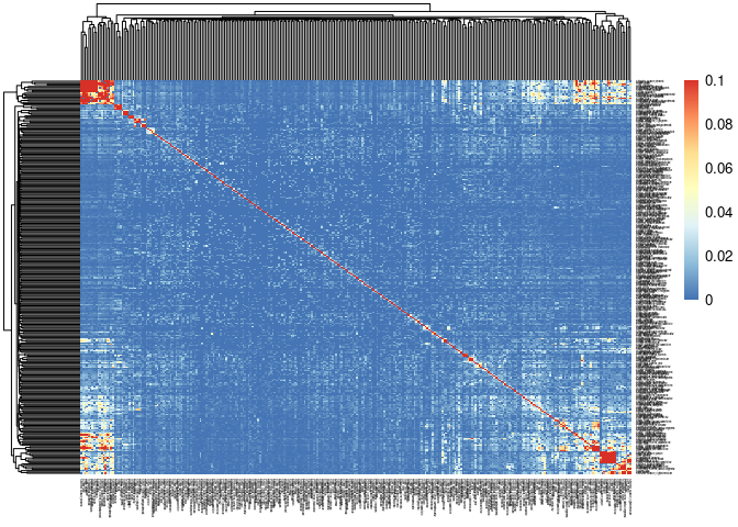

#dev.off()

Fisher’s Exact

P-values were obtained for each overlap to determine which overlapping modules are significant.

## This will create matrices for p-values using Fisher's Exact and a Jaccard Index, which was done above as well
matrix<-matrix(NA,nrow = nrow(mods),ncol = ncol(mods))
p.val<-matrix(NA,nrow = nrow(mods),ncol = ncol(mods))
Jaccard<-matrix(NA,nrow = nrow(mods),ncol = ncol(mods))
for(i in 1:length(rownames(mods))){
  for(j in 1:length(colnames(mods))){
    overlap<-newGeneOverlap(unique(unlist(mylist2[rownames(mods)[i]])),unique(unlist(mylist2[colnames(mods)[j]])))
    overlap2<-testGeneOverlap(overlap)
    Jaccard[i,j]<-getJaccard(overlap2)
    p.val[i,j]<-getPval(overlap2)
  }
}

colnames(p.val)<-colnames(mods)
rownames(p.val)<-rownames(mods)
colnames(Jaccard)<-colnames(mods)
rownames(Jaccard)<-rownames(mods)
        
write.csv(p.val,here("Data","Fisher's_exact_text_p_val_Jaccard_Index_WGCNA_2DG_BL6_Tissue.csv"))
write.csv(Jaccard,here("Data","Jaccard_Index_WGCNA_2DG_BL6_Tissue.csv"))

Jaccard Index Subset

This Jacard Index contains the 4 hotspots identified in the complete jaccard index.

breaks<-seq(0,.5,length.out = 100)

mods <- as.data.frame(mods)
mods.subset <- matrix(nrow = nrow(mods),ncol = ncol(mods))
for(i in 1:length(rownames((mods)))){
  for(j in 1:length(colnames(mods))){
    if(mods[i,j] > 0.08 & mods[i,j] < 1) {mods.subset[i,j] <- mods[i,j]}
    else {mods.subset[i,j]=="NA"}
  }
}

colnames(mods.subset) <- colnames(mods)
rownames(mods.subset) <- rownames(mods)

mods.subset <- mods.subset[rowSums(is.na(mods.subset)) != ncol(mods.subset),]

mods.subset <- as.data.frame(mods.subset) %>%
  rownames_to_column()

mods.subset <- mods.subset[, colSums(is.na(mods.subset)) != nrow(mods.subset)]

mods.subset <- mods.subset %>%
  mutate_all(~replace(., is.na(.), -1))

rownames(mods.subset) <- mods.subset$rowname

mods.subset <-mods.subset[,-1]


pval <- read.csv(here("Data","Fisher's_exact_text_p_val_Jaccard_Index_WGCNA_2DG_BL6_Tissue.csv"), header = T, row.names = 1, check.names = F)

pval <- as.data.frame(pval)

pval.subset <- pval[rownames(pval) %in% rownames(mods.subset),]

pval.subset <- pval.subset[,colnames(pval.subset) %in% colnames(mods.subset)]

#write.csv(pval.subset,here("Data","pval.subset_for_jaccard_module_overlap.csv"))

pval.subset <- read.csv(here("Data","pval.subset_for_jaccard_module_overlap.csv"), row.names = 1, check.names = F)

#pdf("Chang_2DG_BL6_modules_subset_jaccard_0.1.pdf")
pheatmap(mods.subset,cluster_cols=T,cluster_rows=T, fontsize = 10, fontsize_row = 4,fontsize_col = 4,breaks=breaks, display_numbers = pval.subset, fontsize_number = 2, number_format = "%.2f", color = colorRampPalette(brewer.pal(12, "Paired"))(100), number_color = "grey36")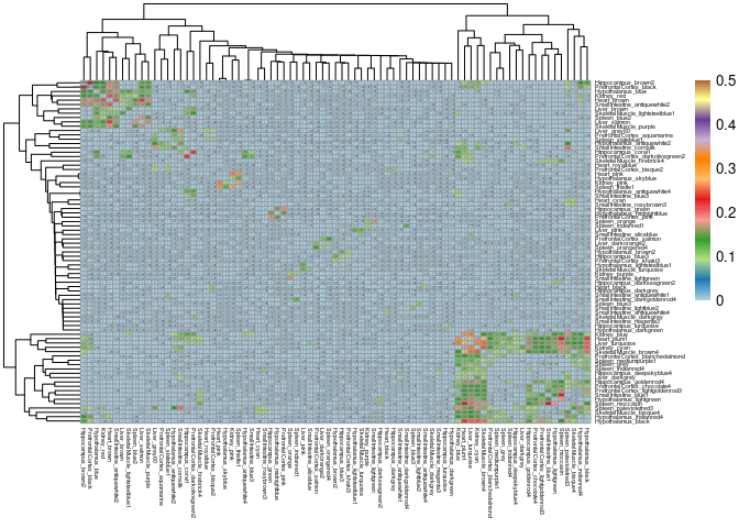

#dev.off()

significant <- c()
header <- c()
        for(i in 1:length(rownames(pval))){ ## This will only pull the significant modules
          for(j in 1:length(colnames(pval))){
            if(pval[i,j] <= 0.05)
            {significant <- c(significant,i,j)
            header <- c(header,paste0(rownames(pval)[i],"_",colnames(pval)[j]))
            }
          }
        }

significant <- matrix(significant,24640,2,TRUE)
header <- matrix(header,24640,1,TRUE)
rownames(significant) <- header

significant2 <- significant[!(significant[,1]==significant[,2]),]
        
shared<-c()
length1<-c()
length2<-c()
length3<-c()

for(i in 1:nrow(significant2)){ ## This creates a list of the rows and columns that correspond to the significant 
  shared[[i]]<-intersect(unlist(mylist2[significant2[i,2]]),unlist(mylist2[significant2[i,1]]))
  length1[[i]]<-length(unlist(mylist2[significant2[i,2]]))
  length2[[i]]<-length(unlist(mylist2[significant2[i,1]]))
  length3[[i]]<-length(intersect(unlist(mylist2[significant2[i,2]]),unlist(mylist2[significant2[i,1]])))
}
names(shared)<-sprintf(rownames(significant2)) ##renames each element of the list

length_bind<-cbind(length2,length1,length3)

saveRDS(length_bind, here("Data","Chang_2DG_BL6_group_length_and_intersection_modules.RData"))
        
ensembl_location<-readRDS(here("Data","Ensembl_gene_id_and_location.RData"))
  
matched_annotation_intersection<-c()
for(i in 1:length(shared)){
  shareddf<-as.data.frame(shared[[i]])
  colnames(shareddf)<-"Genes"
  matched_annotation_intersection[[i]]<-merge(shareddf,ensembl_location,by.x="Genes",by.y="ensembl_gene_id")
}

names(matched_annotation_intersection)<-sprintf(rownames(significant2)) ##renames each element of the list
       
saveRDS(matched_annotation_intersection, here("Data","Chang_2DG_BL6_Matched_annotation_intersection_modules.RData"))
        
Matched<-readRDS(here("Data","Chang_2DG_BL6_Matched_annotation_intersection_modules.RData"))
        
pathway=list()
for(i in 1:length(Matched)){
  gene <- as.vector(Matched[[i]]$Genes)
  profiler <- gost(gene,organism = "mmusculus", correction_method = "fdr", sources = c("KEGG","REAC"))
  #profiler <- gprofiler(gene,organism = "mmusculus", src_filter = c("KEGG","REAC"))
  if(length(profiler) == 0) {pathway[[i]] <- NA}
  else {pathway[[i]] <- profiler$result}
}

names(pathway)<-sprintf(names(Matched)) ##renames each element of the list

saveRDS(pathway,here("Data","Chang_2DG_BL6_gprofiler_annotation_list_modules.RData"))

pathways.jaccard <- readRDS(here("Data","Chang_2DG_BL6_gprofiler_annotation_list_modules.RData"))

filtered.pathways <- pathways.jaccard[!is.na(pathways.jaccard)]

saveRDS(filtered.pathways,here("Data","Chang_2DG_BL6_gprofiler_annotation_filtered_list_modules.RData"))

Pathway Analysis

Pathway analysis was performed using the gprofiler package. Genes associated with each module were compared against KEGG and REACTOME databases. Each pathway listed represents the pathways shared among the two modules. All modules represented were significantly overlapped and all pathways represented are significant according to their adjusted p-value (FDR < 0.05).

filtered.pathways <- readRDS(here("Data","Chang_2DG_BL6_gprofiler_annotation_filtered_list_modules.RData"))

# for(i in 1:length(filtered.pathways)){
#   cat("\n###",names(filtered.pathways)[i], "Module","\n")
#   print(knitr::kable(filtered.pathways[[i]][c(11,3:6)], format = "markdown", col.names = c("Pathway","Raw p-value","Term Size", "Query Size", "Overlap Size")))
# 
#   #print(DT::datatable(filter.pathways[[i]][c(12,3:6)], colnames=c("Pathway"="term.name","Raw p-value"="p.value","Term Size"="term.size", "Query Size"="query.size", "Overlap Size"="overlap.size"), filter = "bottom", style="bootstrap"))
#   cat("\n \n")
# }

Pathway Frequency

The number of times each pathway was identified across pairwise overlaps was counted and listed below.

filtered.pathways <- readRDS(here("Data","Chang_2DG_BL6_gprofiler_annotation_filtered_list_modules.RData"))

list.pathways <- list()
  for(i in 1:length(filtered.pathways)){
    if(class(filtered.pathways[[i]]) == "numeric") {next}
    else {list.pathways[[i]] <- filtered.pathways[[i]]$term_name}
  }
  
  list.pathways <- unlist(list.pathways)
  
  count <- as.data.frame(table(list.pathways)) %>% arrange(desc(Freq))

Frequency Plot

  #pdf("Counts_of_each_pathway_identified_within_jaccard_index.pdf")
  p <- ggplot(data=count,aes(x=list.pathways,y=Freq))
  p <- p + geom_bar(color="black", fill=colorRampPalette(brewer.pal(n = 12, name = "Paired"))(length(count[,1])), stat="identity",position="identity") + theme_classic()
  p <- p + theme(axis.text.x = element_text(angle = 90, hjust =1, size = 3)) + scale_x_discrete(labels=count$list.pathways) + xlab("Modules")
  print(p)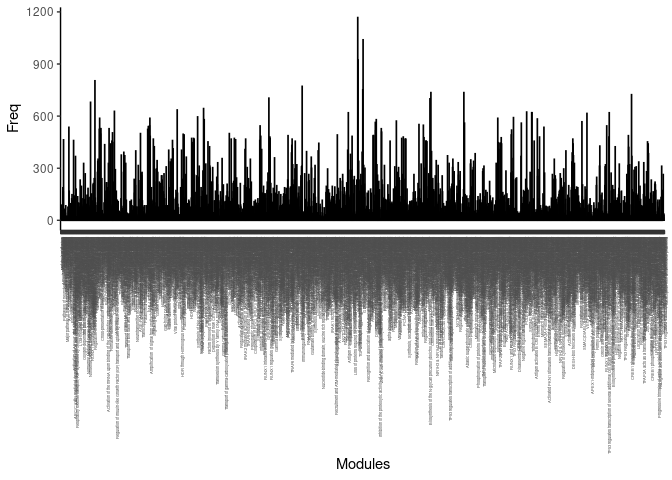

  #dev.off()

Frequency Table

DT::datatable(count, colnames = c("Pathway", "Frequency"), extensions = 'Buttons',
                                           rownames = FALSE, 
                                           filter="top",
                                           options = list(dom = 'Blfrtip',
                                                          buttons = c('copy', 'csv', 'excel'),
                                                          lengthMenu = list(c(10,25,50,-1),
                                                                            c(10,25,50,"All")), 
                                                          scrollX= TRUE), class = "display")

Analysis performed by Ann Wells

The Carter Lab The Jackson Laboratory 2023

ann.wells@jax.org

Jaccard Indeces Comparing WGCNA Modules Across Tissues

Ann Wells

April 23, 2023