Module Generation Heart
Ann Wells
April 23, 2023
log.tdata.FPKM.sample.info.subset.heart.WGCNA <- readRDS(here("Data","Heart","log.tdata.FPKM.sample.info.subset.heart.missing.WGCNA.RData"))Set Up Environment
The WGCNA package requires some strict R session environment set up.
options(stringsAsFactors=FALSE)

# Run the following only if running from terminal
# Does NOT work in RStudio
#enableWGCNAThreads()
Choosing Soft-Thresholding Power
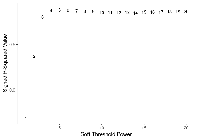
WGCNA uses a smooth softmax function to force a scale-free topology on the gene expression network. I cycled through a set of threshold power values to see which one is the best for the specific topology. As recommended by the authors, I choose the smallest power such that the scale-free topology correlation attempts to hit 0.9.
threshold <- softthreshold(soft)Scale Free Topology
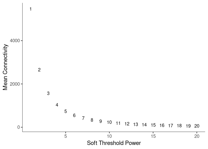
Mean Connectivity
Pick Soft Threshold
knitr::kable(soft$fitIndices)| Power | SFT.R.sq | slope | truncated.R.sq | mean.k. | median.k. | max.k. |
|---|---|---|---|---|---|---|
| 1 | 0.3135009 | 0.9084004 | 0.4860802 | 5474.52077 | 5276.544976 | 8294.7573 |
| 2 | 0.3723904 | -0.3819636 | 0.2861740 | 2651.44036 | 2247.471737 | 5538.8915 |
| 3 | 0.8015318 | -0.7166151 | 0.7453908 | 1565.36846 | 1132.283543 | 4204.3747 |
| 4 | 0.8730707 | -0.8490528 | 0.8372420 | 1035.89223 | 638.190780 | 3402.0568 |
| 5 | 0.8805814 | -0.9393276 | 0.8466313 | 737.27705 | 388.316952 | 2869.1864 |
| 6 | 0.8773132 | -0.9976829 | 0.8438473 | 551.52983 | 247.742555 | 2476.0903 |
| 7 | 0.8714931 | -1.0374971 | 0.8412314 | 427.66727 | 164.606127 | 2171.3506 |
| 8 | 0.8662610 | -1.0662577 | 0.8407856 | 340.71318 | 113.593305 | 1926.8744 |
| 9 | 0.8645393 | -1.0925861 | 0.8459215 | 277.22370 | 80.647333 | 1725.7984 |
| 10 | 0.8511895 | -1.1172364 | 0.8393946 | 229.41409 | 58.234409 | 1557.2606 |
| 11 | 0.8550061 | -1.1313784 | 0.8508515 | 192.50713 | 43.014165 | 1413.8767 |
| 12 | 0.8507925 | -1.1491267 | 0.8535778 | 163.43002 | 32.462611 | 1290.4119 |
| 13 | 0.8527970 | -1.1597074 | 0.8623260 | 140.12825 | 24.721304 | 1183.0293 |
| 14 | 0.8481418 | -1.1762096 | 0.8631199 | 121.18296 | 18.956198 | 1088.8396 |
| 15 | 0.8565609 | -1.1809611 | 0.8754847 | 105.58711 | 14.762382 | 1005.6185 |
| 16 | 0.8568787 | -1.1899092 | 0.8819458 | 92.60907 | 11.741628 | 931.6209 |
| 17 | 0.8558067 | -1.2003995 | 0.8855642 | 81.70638 | 9.369532 | 865.4564 |
| 18 | 0.8606257 | -1.2084899 | 0.8918230 | 72.46974 | 7.568808 | 806.0016 |
| 19 | 0.8609341 | -1.2181280 | 0.8958867 | 64.58547 | 6.174519 | 752.3379 |
| 20 | 0.8646870 | -1.2237273 | 0.9014236 | 57.80986 | 5.001578 | 703.7069 |
soft$fitIndices %>%
  download_this(
    output_name = "Soft Threshold Heart",
    output_extension = ".csv",
    button_label = "Download data as csv",
    button_type = "info",
    has_icon = TRUE,
    icon = "fa fa-save"
)Calculate Adjacency Matrix and Topological Overlap Matrix
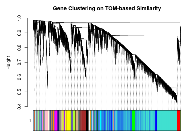
I generated a weighted adjacency matrix for the gene expression profile network using the softmax threshold I determined in the previous step. Then I generate the Topological Overlap Matrix (TOM) for the adjacency matrix. This reduces noise and spurious associations according to the authors.I use the TOM matrix to cluster the profiles of each metabolite based on their similarity. I use dynamic tree cutting to generate modules.
soft.power <- which(soft$fitIndices$SFT.R.sq >= 0.88)[1]
cat("\n", "Power chosen")
##
## Power chosensoft.power## [1] 5cat("\n \n")adj.mtx <- adjacency(log.tdata.FPKM.sample.info.subset.heart.WGCNA, power=soft.power)
TOM = TOMsimilarity(adj.mtx)## ..connectivity..
## ..matrix multiplication (system BLAS)..
## ..normalization..
## ..done.diss.TOM = 1 - TOM
metabolite.clust <- hclust(as.dist(diss.TOM), method="average")
min.module.size <- 15
modules <- cutreeDynamic(dendro=metabolite.clust, distM=diss.TOM, deepSplit=2, pamRespectsDendro=FALSE, minClusterSize=min.module.size)## ..cutHeight not given, setting it to 0.983 ===> 99% of the (truncated) height range in dendro.
## ..done.#saveRDS(modules,here("Data","Heart","Chang_2DG_BL6_modules_heart.RData"))
# Plot modules
cols <- labels2colors(modules)
table(cols)## cols
## black blue brown cyan darkgreen
## 386 2132 935 227 138
## darkgrey darkmagenta darkolivegreen darkorange darkred
## 127 76 77 109 140
## darkturquoise green greenyellow grey60 lightcyan
## 135 459 274 191 198
## lightcyan1 lightgreen lightsteelblue1 lightyellow magenta
## 27 188 28 181 311
## mediumpurple3 midnightblue orange orangered4 paleturquoise
## 29 219 116 48 92
## pink plum1 purple red royalblue
## 381 56 298 392 144
## saddlebrown salmon sienna3 skyblue skyblue3
## 97 231 73 98 66
## steelblue tan turquoise violet white
## 94 266 7088 81 103
## yellow yellowgreen
## 853 72plotDendroAndColors(
metabolite.clust, cols, xlab="", sub="", main="Gene Clustering on TOM-based Similarity",
dendroLabels=FALSE, hang=0.03, addGuide=TRUE, guideHang=0.05
)
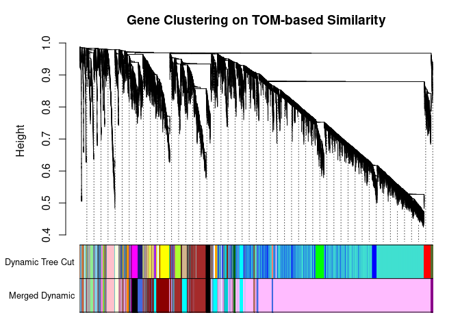
Merging Related Modules
Some modules might be highly correlated. The authors recommend merging modules with a correlation greater than 0.75.
me.list <- moduleEigengenes(log.tdata.FPKM.sample.info.subset.heart.WGCNA, colors=cols)
me <- me.list$eigengenes

# Eigenmetabolite dissimilarity
me.diss <- 1 - cor(me)

h <- hclust(as.dist(me.diss), method="average")

# Merge threshold = 1 - correlation threshold
merge.thresh <- 0.25

plot(h, main="Clustering of Module Eigengene", xlab="", sub="")
abline(h=merge.thresh, col="red")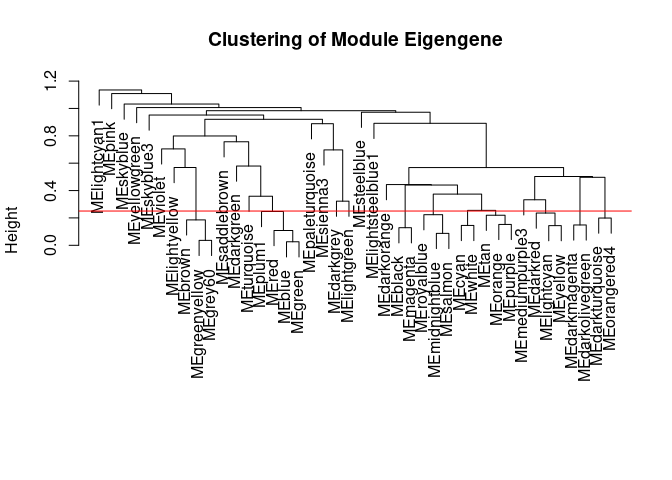
merge <- mergeCloseModules(log.tdata.FPKM.sample.info.subset.heart.WGCNA, cols, cutHeight=merge.thresh, verbose=0)
merged.cols <- merge$colors
merged.mes <- merge$newMEs

  # Check how the merging changed the clustering of the metabolites
plotDendroAndColors(
  metabolite.clust, cbind(cols, merged.cols), c("Dynamic Tree Cut", "Merged Dynamic"), xlab="", sub="",
  main="Gene Clustering on TOM-based Similarity",
  dendroLabels=FALSE, hang=0.03, addGuide=TRUE, guideHang=0.05
  )
Calculating Intramodular Connectivity
This function in WGCNA calculates the total connectivity of a node (metabolite) in the network. The kTotal column specifies this connectivity. The kWithin column specifies the node connectivity within its module. The kOut column specifies the difference between kTotal and kWithin. Generally, the out degree should be lower than the within degree, since the WGCNA procedure groups similar metabolite profiles together.
net.deg <- intramodularConnectivity(adj.mtx, merged.cols)
saveRDS(net.deg,here("Data","Heart","Chang_2DG_BL6_connectivity_heart.RData"))
head(net.deg)
## kTotal kWithin kOut kDiff
## ENSMUSG00000000001 415.44248 95.369953 320.07253 -224.70257
## ENSMUSG00000000028 61.89615 9.291988 52.60416 -43.31217
## ENSMUSG00000000031 289.27483 171.650109 117.62472 54.02539
## ENSMUSG00000000037 52.92083 4.641655 48.27917 -43.63752
## ENSMUSG00000000049 179.43989 96.973970 82.46592 14.50805
## ENSMUSG00000000056 801.97669 764.017184 37.95950 726.05768Summary
The dataset generated coexpression modules of the following sizes. The grey submodule represents metabolites that did not fit well into any of the modules.
table(merged.cols)## merged.cols
## black brown cyan darkgreen darkgrey
## 697 1400 1010 138 127
## darkmagenta darkorange darkred darkturquoise lightcyan1
## 153 109 1191 183 27
## lightgreen lightsteelblue1 lightyellow mediumpurple3 paleturquoise
## 188 28 181 29 92
## pink plum1 royalblue saddlebrown sienna3
## 381 10127 594 97 73
## skyblue skyblue3 steelblue violet yellowgreen
## 98 66 94 81 72# Module names in descending order of size
module.labels <- names(table(merged.cols))[order(table(merged.cols), decreasing=T)]
#saveRDS(module.labels,here("Data","Heart","Chang_2DG_BL6_module_labels_heart.RData"))
# Order eigenmetabolites by module labels
merged.mes <- merged.mes[,paste0("ME", module.labels)]
colnames(merged.mes) <- paste0("log.tdata.FPKM.sample.info.subset.heart.WGCNA_", module.labels)
module.eigens <- merged.mes
# Add log.tdata.FPKM.sample.info.subset.WGCNA tag to labels
module.labels <- paste0("log.tdata.FPKM.sample.info.subset.heart.WGCNA_", module.labels)
# Generate and store metabolite membership
module.membership <- data.frame(
Gene=colnames(log.tdata.FPKM.sample.info.subset.heart.WGCNA),
Module=paste0("log.tdata.FPKM.sample.info.subset.heart.WGCNA_", merged.cols)
)
saveRDS(module.labels, here("Data","Heart","log.tdata.FPKM.sample.info.subset.heart.WGCNA.module.labels.RData"))
saveRDS(module.eigens, here("Data","Heart","log.tdata.FPKM.sample.info.subset.heart.WGCNA.module.eigens.RData"))
saveRDS(module.membership, here("Data","Heart", "log.tdata.FPKM.sample.info.subset.heart.WGCNA.module.membership.RData"))
write.table(module.labels, here("Data","Heart","log.tdata.FPKM.sample.info.subset.heart.WGCNA.module.labels.csv"), row.names=F, col.names=F, sep=",")
write.csv(module.eigens, here("Data","Heart","log.tdata.FPKM.sample.info.subset.heart.WGCNA.module.eigens.csv"))
write.csv(module.membership, here("Data","Heart","log.tdata.FPKM.sample.info.subset.heart.WGCNA.module.membership.csv"), row.names=F)Analysis performed by Ann Wells
The Carter Lab The Jackson Laboratory 2023
ann.wells@jax.org