Module Sample Contribution Skeletal Muscle
Ann Wells
April 23, 2023
Introduction and Data files
R Markdown
This dataset contains nine tissues (heart, hippocampus, hypothalamus, kidney, liver, prefrontal cortex, skeletal muscle, small intestine, and spleen) from C57BL/6J mice that were fed 2-deoxyglucose (6g/L) through their drinking water for 96hrs or 4wks. 96hr mice were given their 2DG treatment 2 weeks after the other cohort started the 4 week treatment. The organs from the mice were harvested and processed for metabolomics and transcriptomics. The data in this document pertains to the transcriptomics data only. The counts that were used were FPKM normalized before being log transformed. It was determined that sample A113 had low RNAseq quality and through further analyses with PCA, MA plots, and clustering was an outlier and will be removed for the rest of the analyses performed. This document will determine how samples are contributing to each module.
needed.packages <- c("tidyverse", "here", "functional", "gplots", "dplyr", "GeneOverlap", "R.utils", "reshape2","magrittr","data.table", "RColorBrewer","preprocessCore", "ARTool","emmeans", "phia", "gProfileR","pheatmap")
for(i in 1:length(needed.packages)){library(needed.packages[i], character.only = TRUE)}

source(here("source_files","WGCNA_source.R"))
source(here("source_files","plot_theme.R"))
tdata.FPKM.sample.info <- readRDS(here("Data","20190406_RNAseq_B6_4wk_2DG_counts_phenotypes.RData"))
tdata.FPKM <- readRDS(here("Data","20190406_RNAseq_B6_4wk_2DG_counts_numeric.RData"))
log.tdata.FPKM <- log(tdata.FPKM + 1)
log.tdata.FPKM <- as.data.frame(log.tdata.FPKM)
log.tdata.FPKM.sample.info <- cbind(log.tdata.FPKM, tdata.FPKM.sample.info[,27238:27240])
log.tdata.FPKM.sample.info <- log.tdata.FPKM.sample.info %>% rownames_to_column() %>% filter(rowname != "A113") %>% column_to_rownames()
log.tdata.FPKM.subset <- log.tdata.FPKM[,colMeans(log.tdata.FPKM != 0) > 0.5]
log.tdata.FPKM.sample.info.subset <- cbind(log.tdata.FPKM.subset,tdata.FPKM.sample.info[,27238:27240])
log.tdata.FPKM.sample.info.subset <- log.tdata.FPKM.sample.info.subset %>% rownames_to_column() %>% filter(rowname != "A113") %>% column_to_rownames()
log.tdata.FPKM.sample.info.subset.muscle <- log.tdata.FPKM.sample.info.subset %>% rownames_to_column() %>% filter(Tissue == "Skeletal Muscle") %>% column_to_rownames()
modules <- read.csv(here("Data","Skeletal Muscle","log.tdata.FPKM.sample.info.subset.skeletal.muscle.WGCNA.module.membership.csv"), header=T)
eigens <- read.csv(here("Data","Skeletal Muscle","log.tdata.FPKM.sample.info.subset.skeletal.muscle.WGCNA.module.eigens.csv"), header=T)Module Sample Contribution
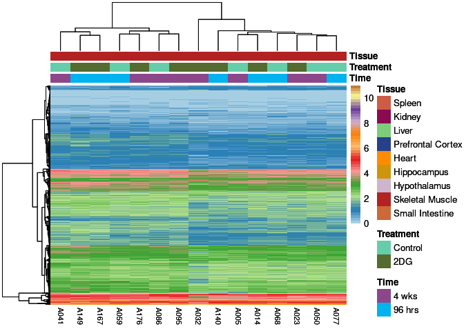
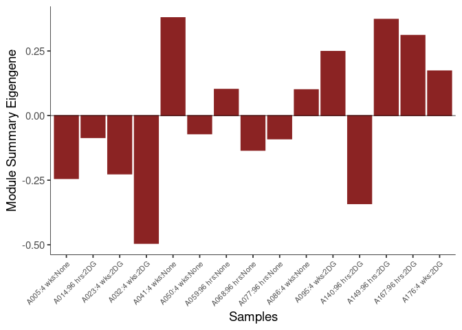
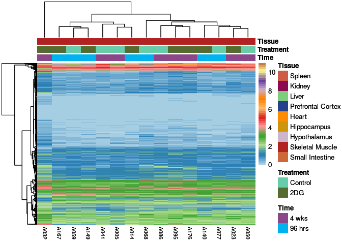
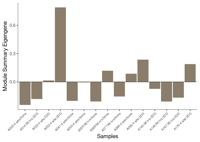
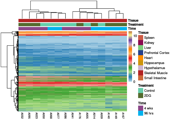
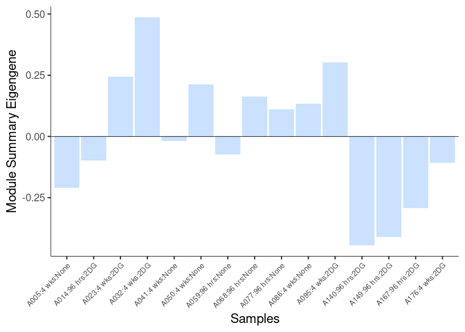
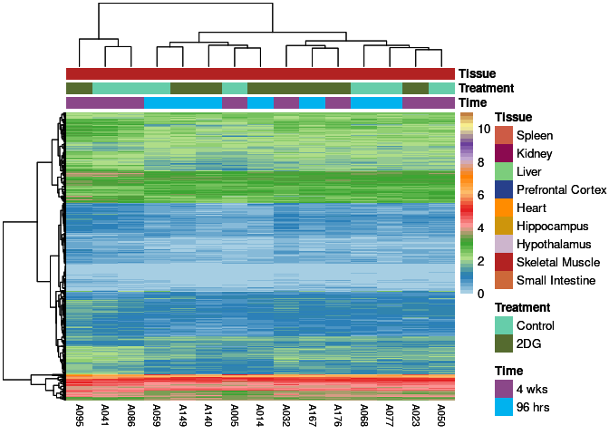
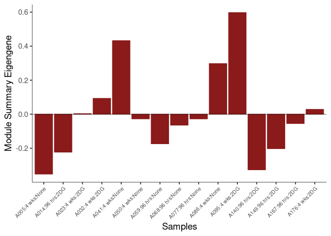
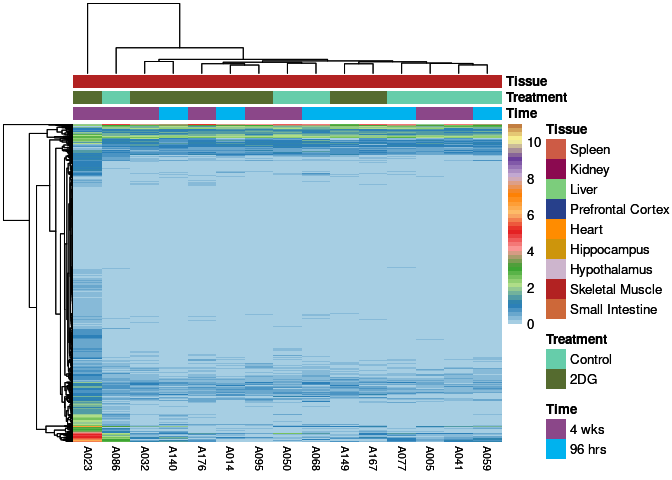
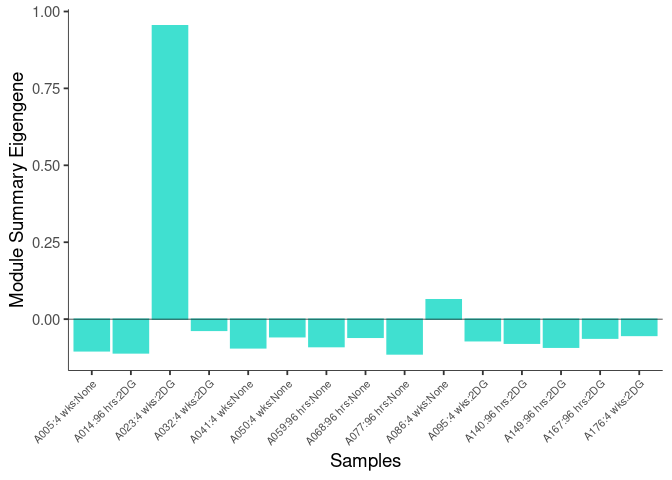
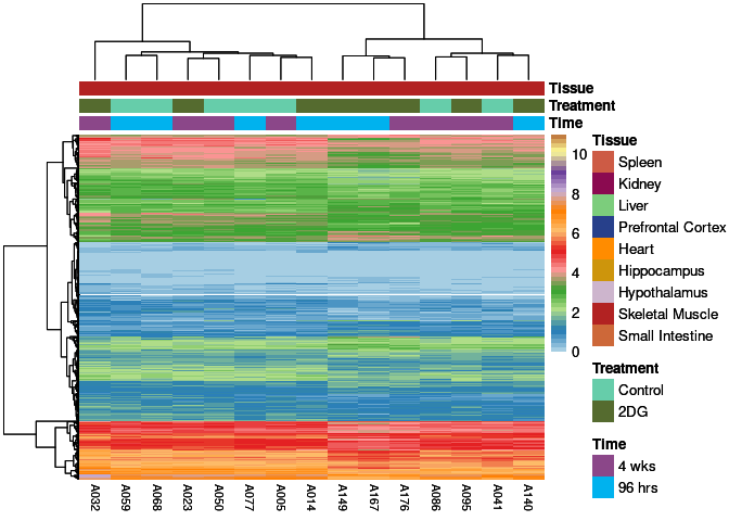
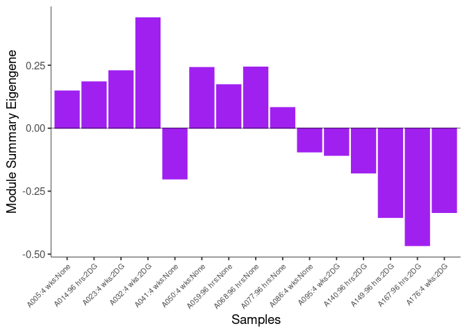
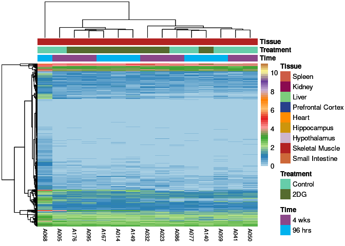
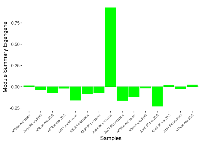
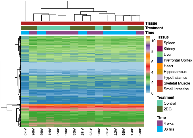
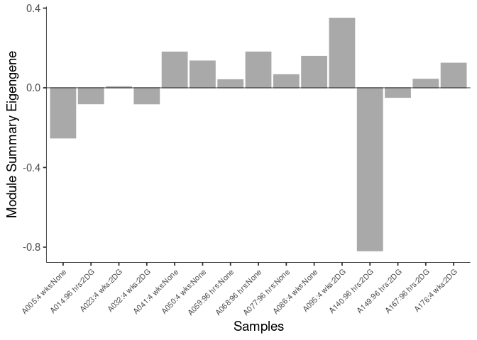
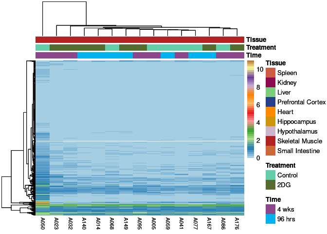
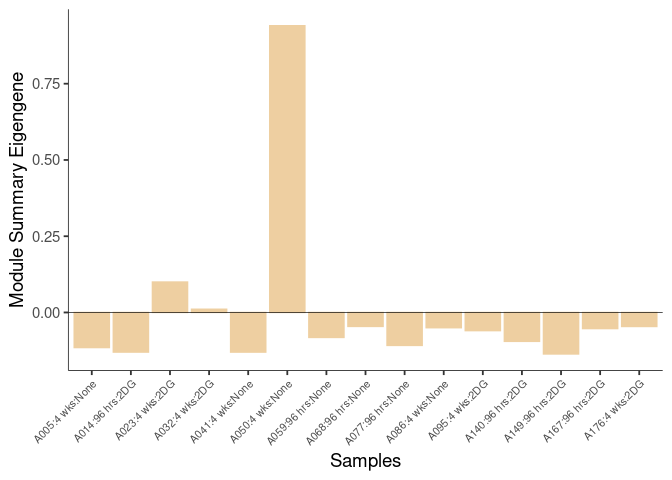
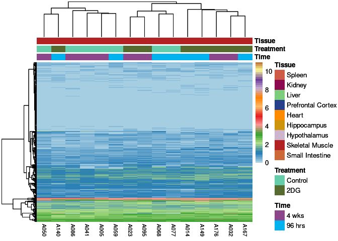
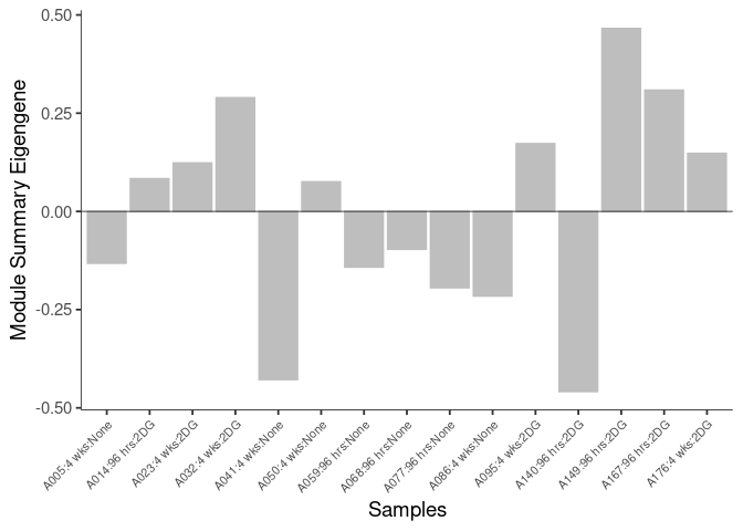
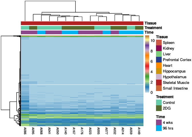
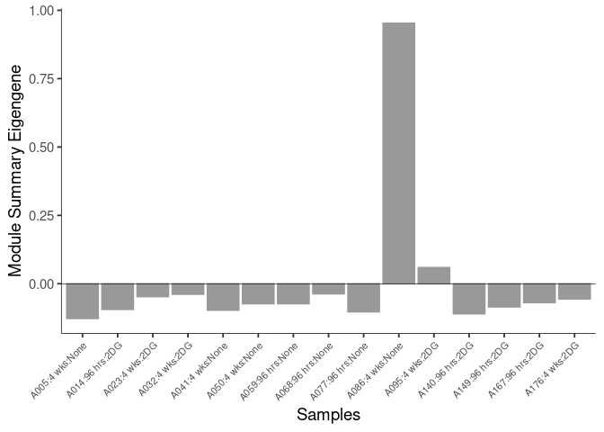
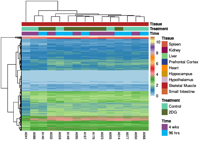
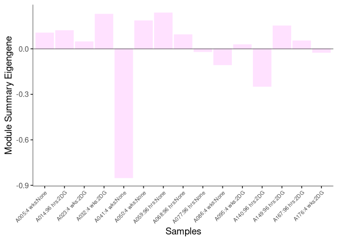
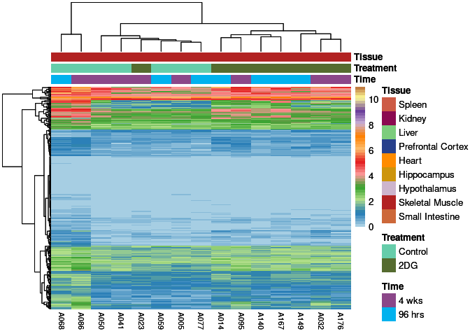
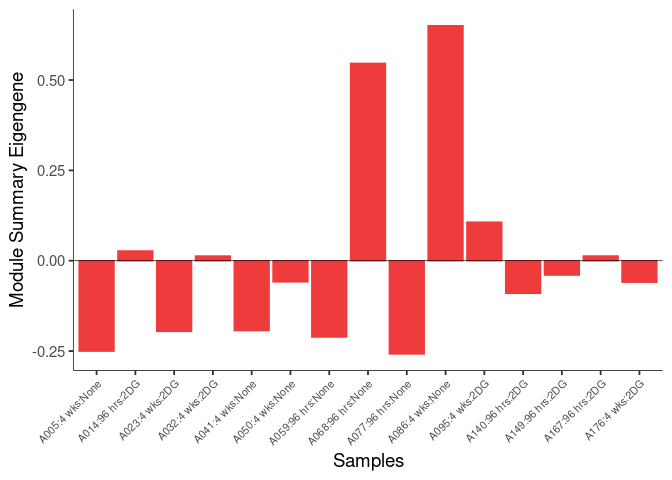
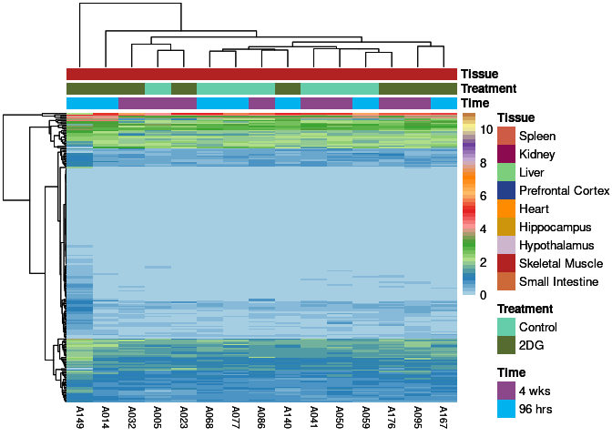
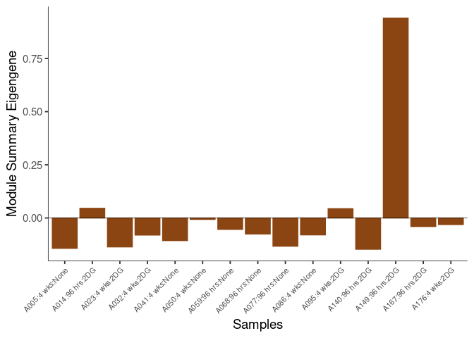
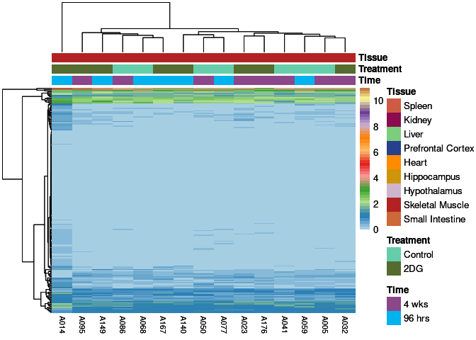
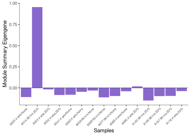
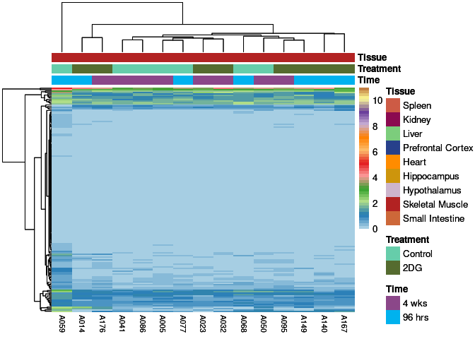
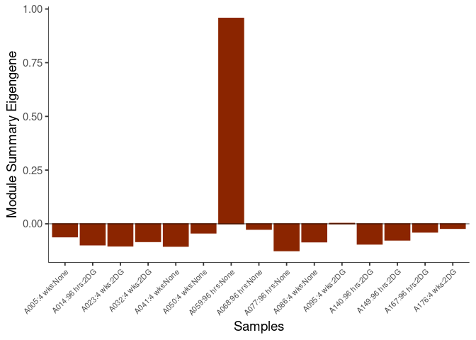
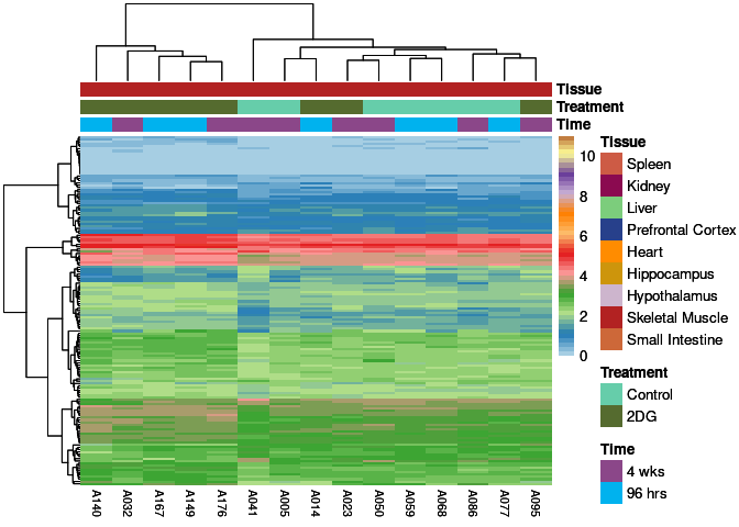
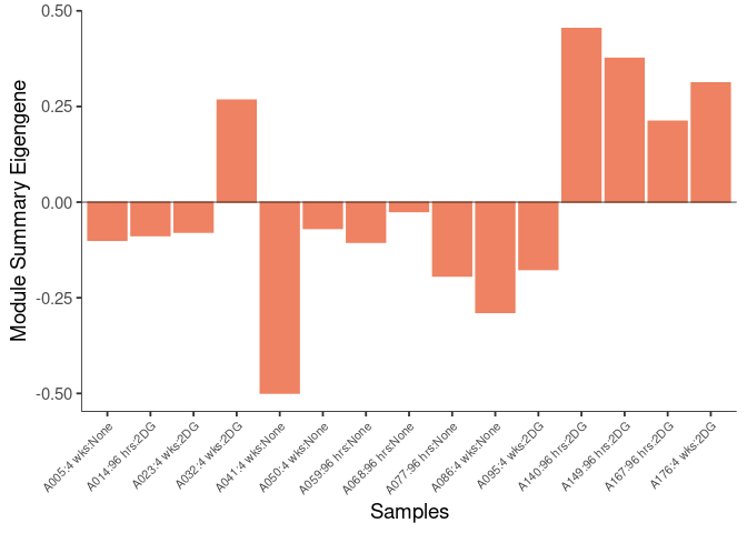
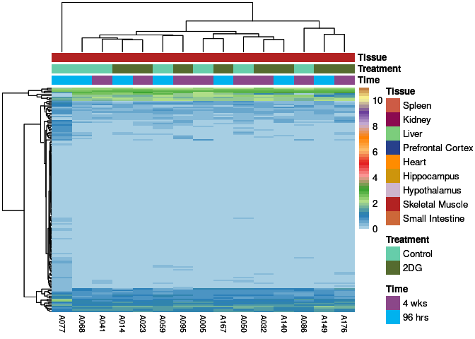
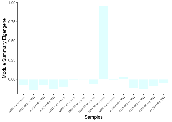
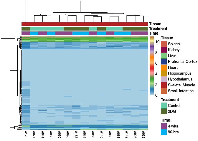
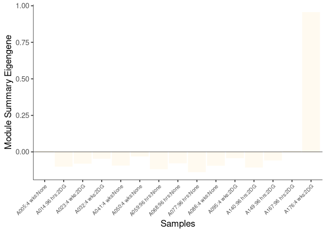
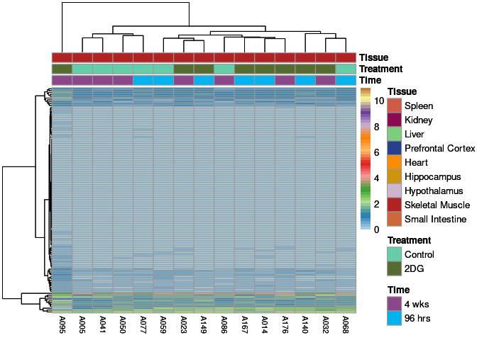
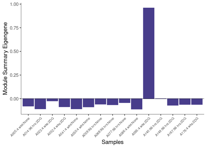
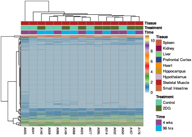
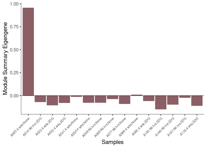
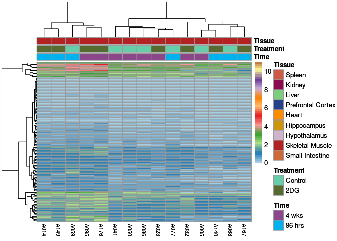
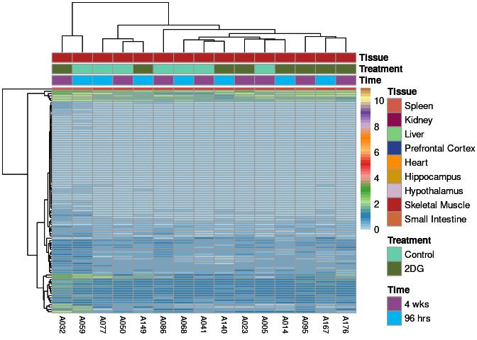
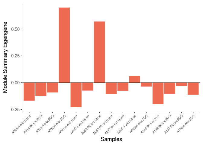
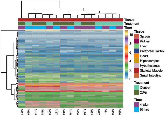
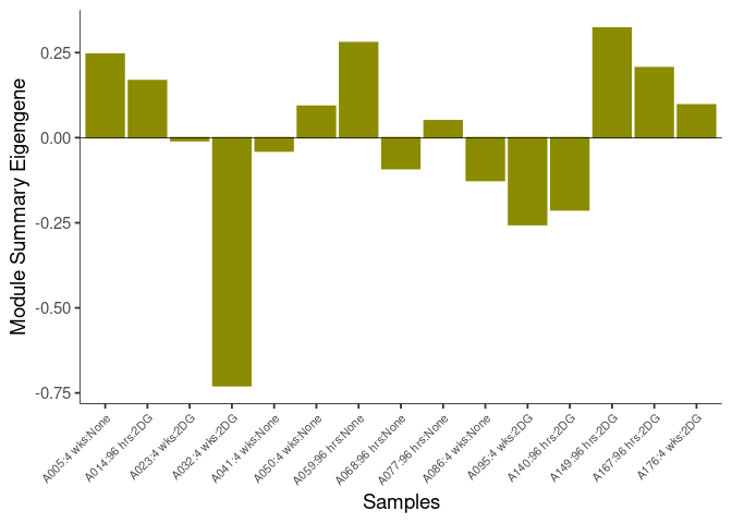
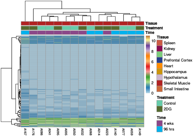
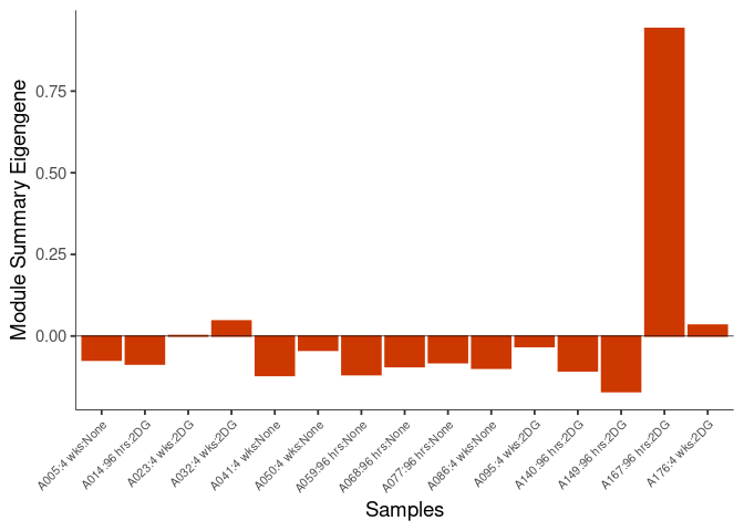
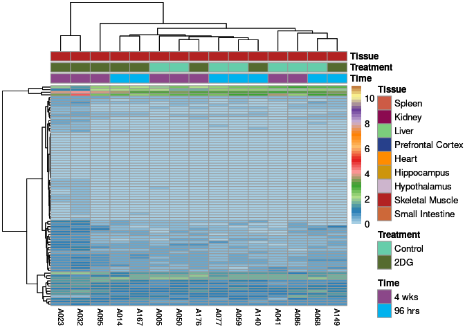
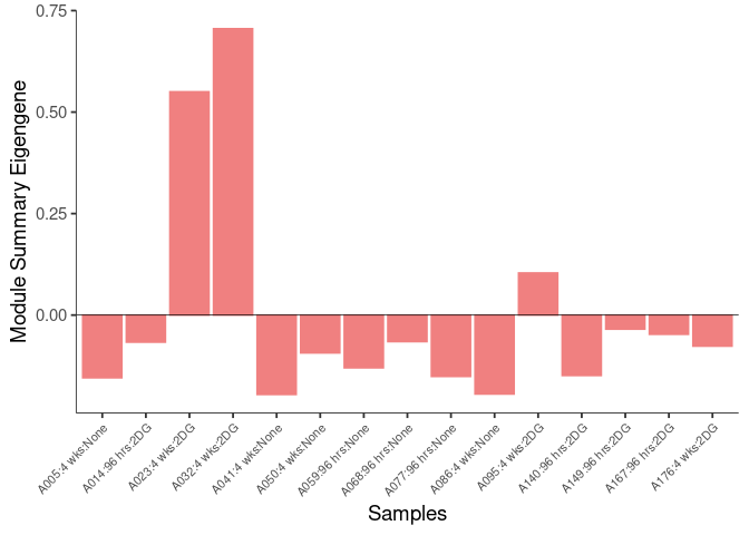
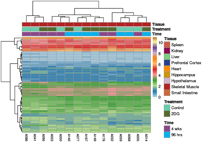
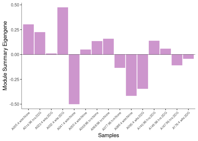
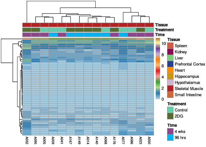
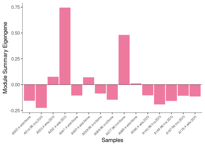
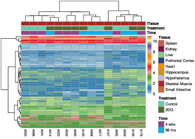
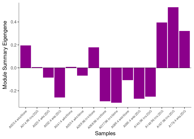
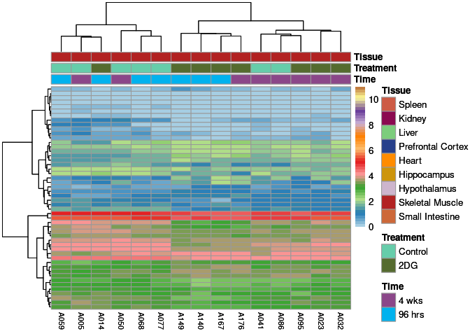
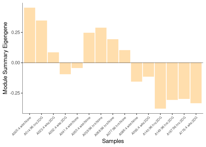
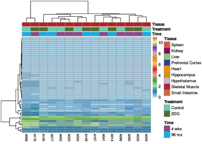
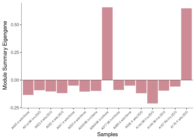
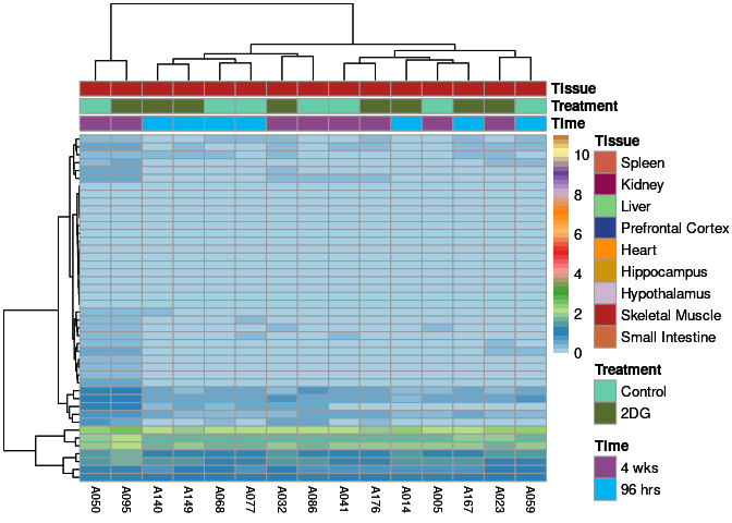
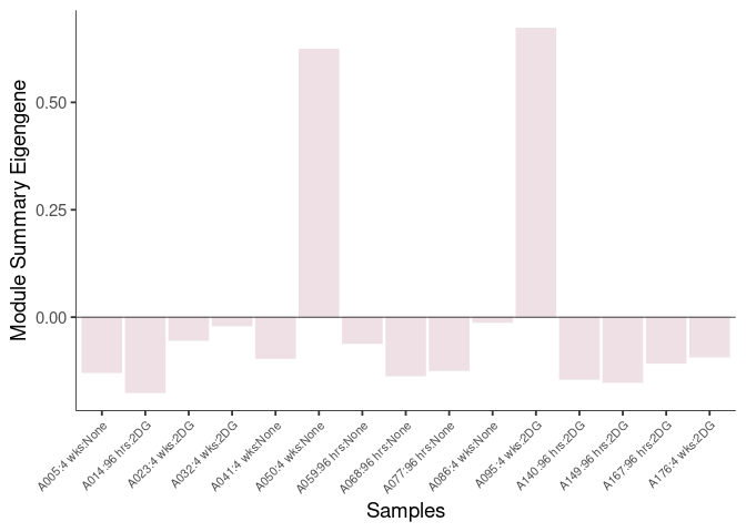
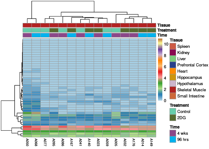
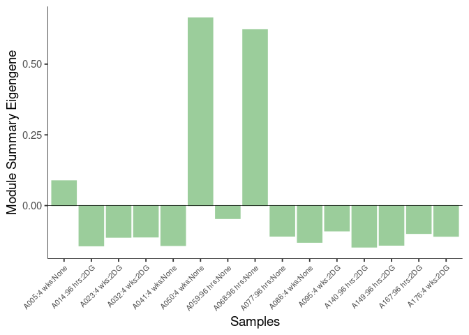
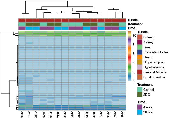
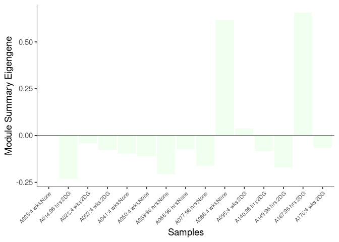
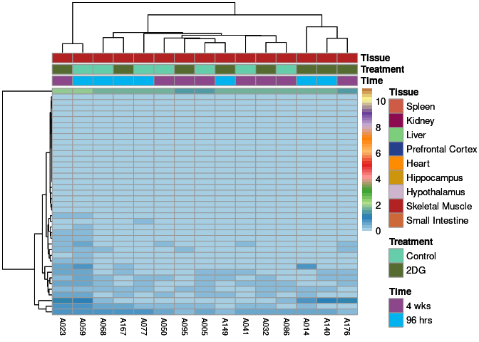
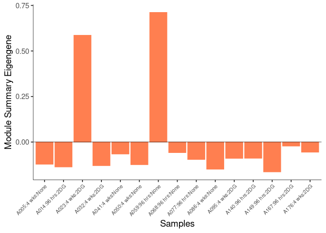
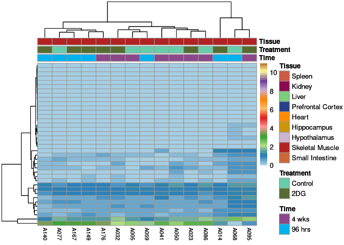
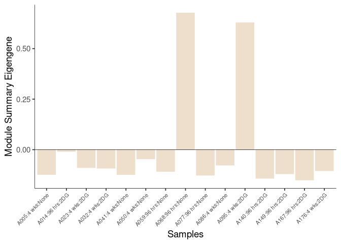
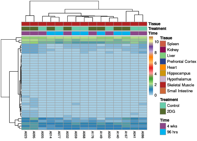
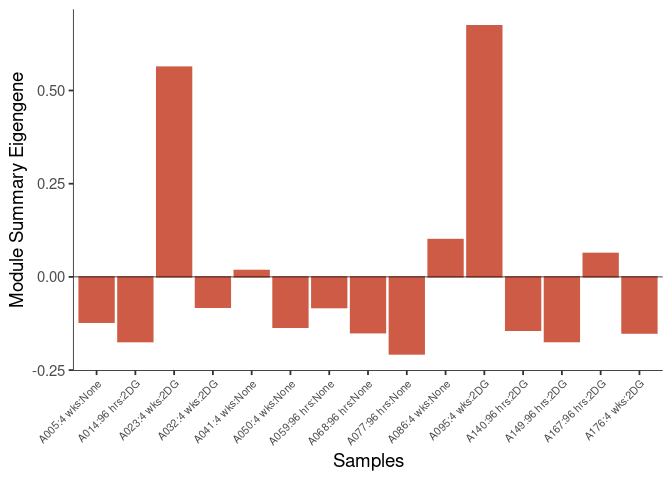
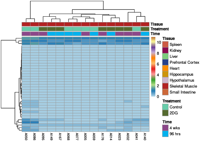
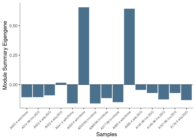
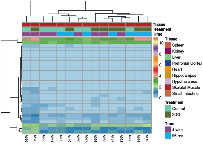
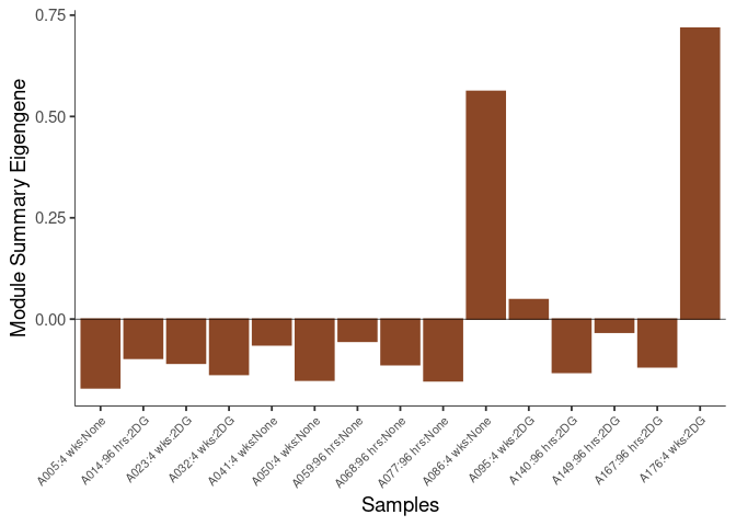
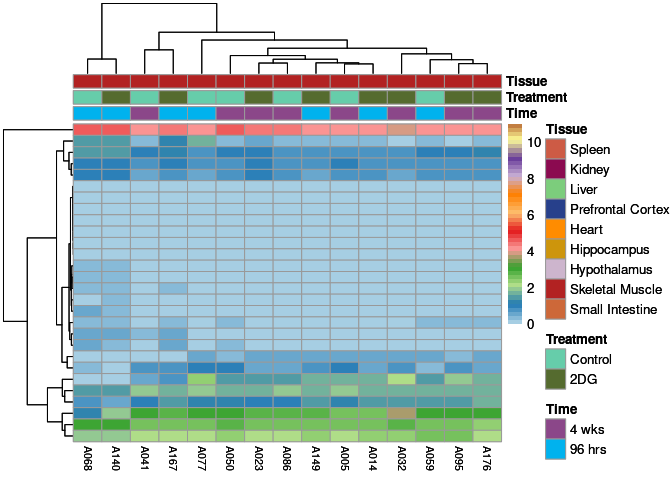
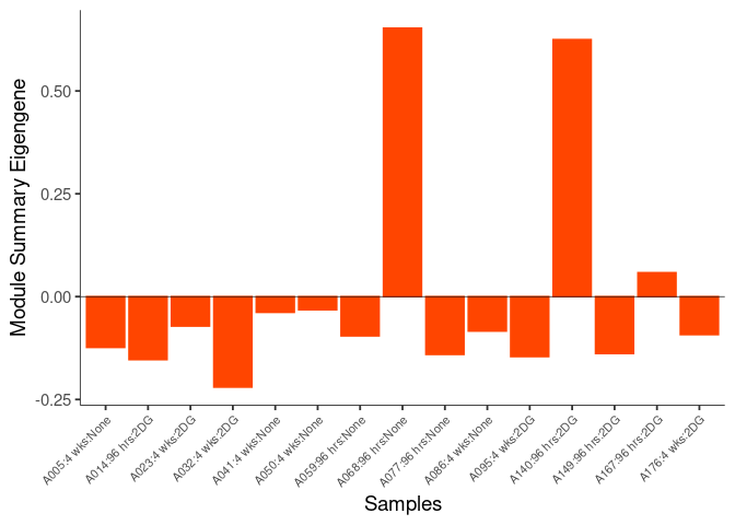
The heatmap shows the expression level of each gene in the module across all samples present in this subsetted dataset. The bar plot shows the relative eigen value summarizing gene expression for each sample present in this subsetted dataset.
eigen.expression(eigens,log.tdata.FPKM.sample.info.subset.muscle)brown4 Module
bisque4 Module
lightsteelblue1 Module
firebrick4 Module
turquoise Module
purple Module
green Module
darkgrey Module
navajowhite2 Module
grey Module
grey60 Module
thistle1 Module
brown2 Module
saddlebrown Module
mediumpurple3 Module
orangered4 Module
salmon2 Module
lightcyan1 Module
floralwhite Module
darkslateblue Module
lightpink4 Module
honeydew1 Module

coral2 Module
yellow4 Module
orangered3 Module
lightcoral Module
plum3 Module
palevioletred2 Module
magenta4 Module
navajowhite1 Module
lightpink3 Module
lavenderblush2 Module
darkseagreen3 Module
honeydew Module
coral Module
antiquewhite2 Module
coral3 Module
skyblue4 Module
sienna4 Module
orangered1 Module
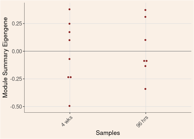
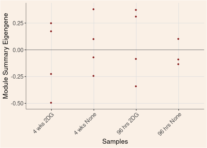
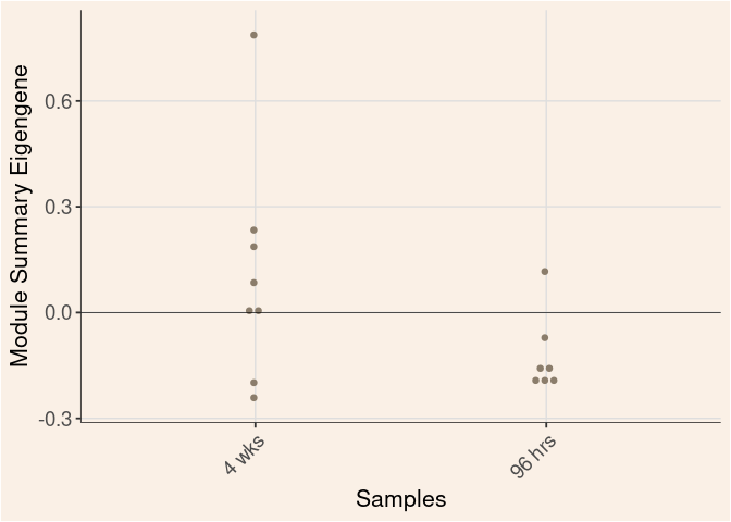
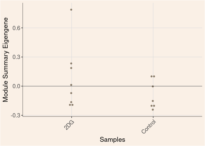
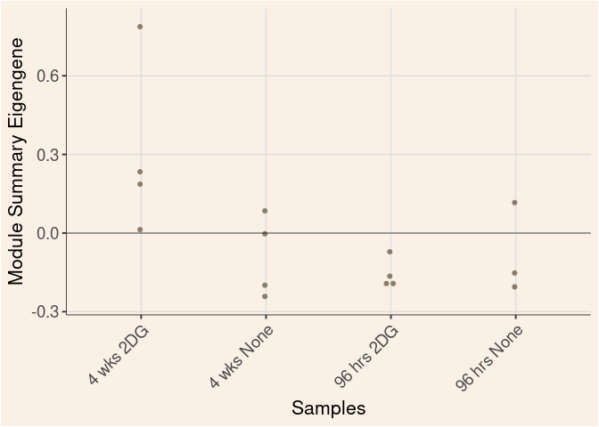
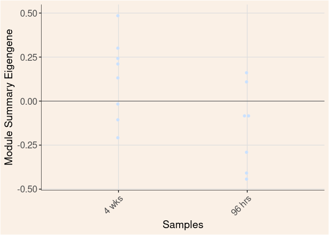
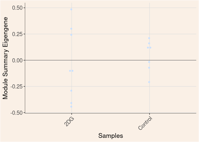
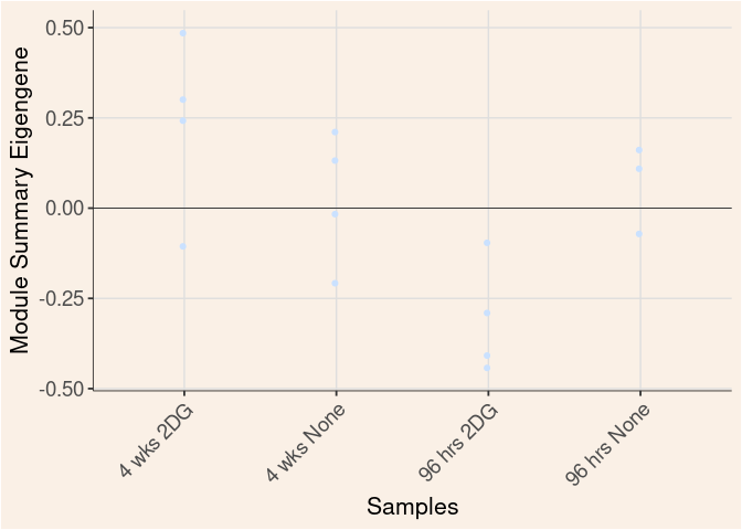
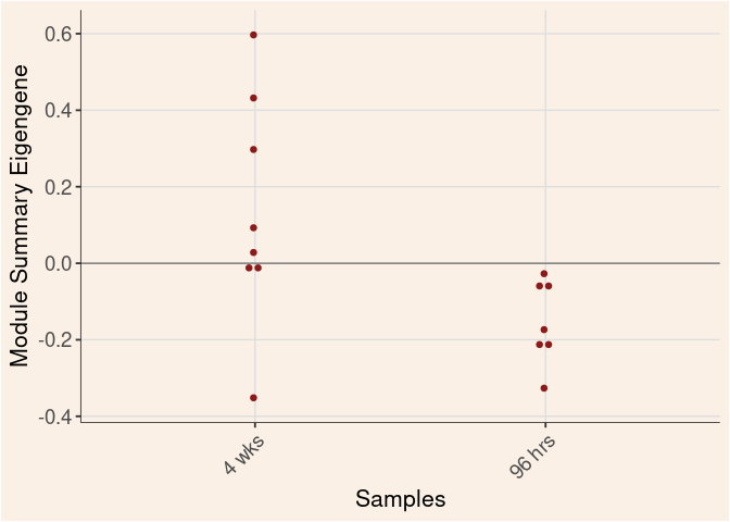
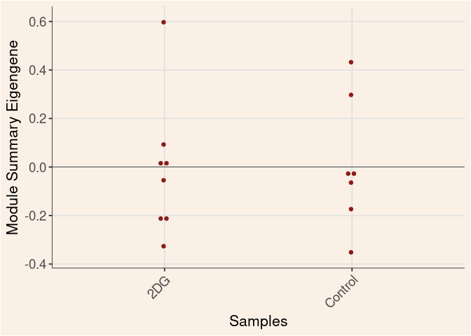
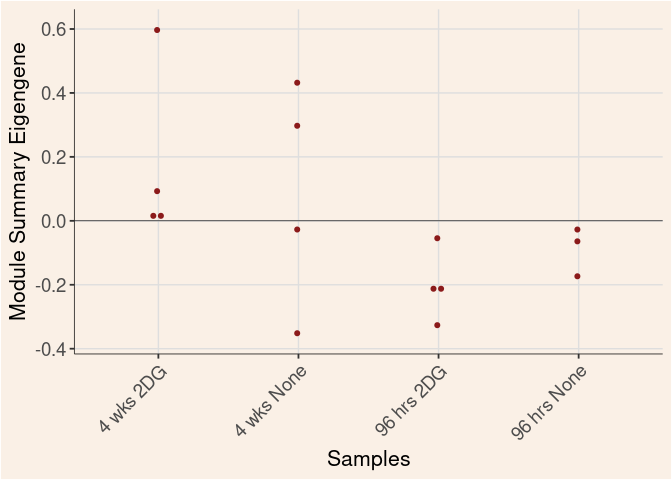
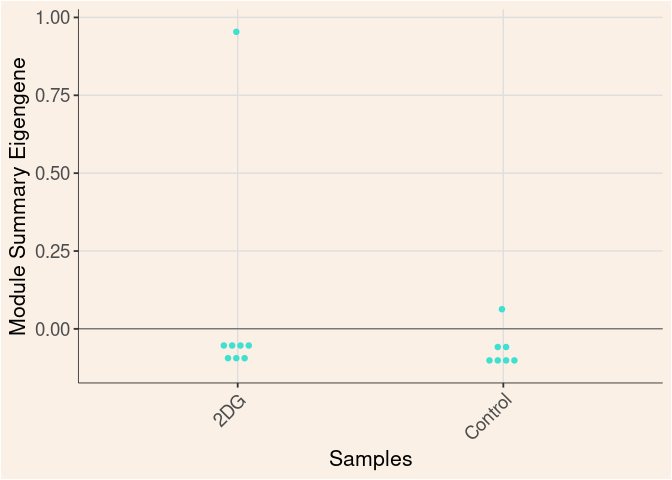
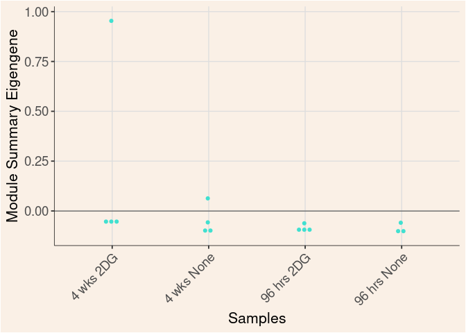
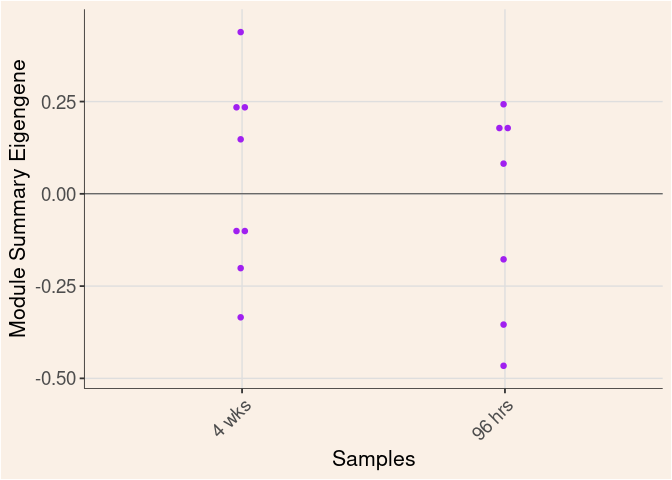
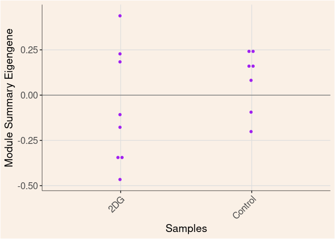
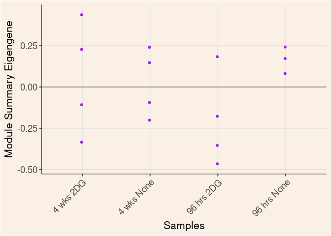
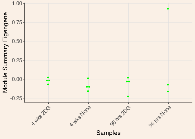
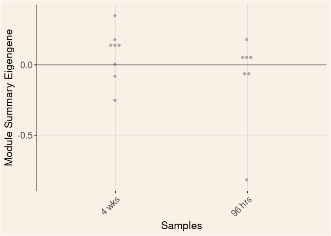
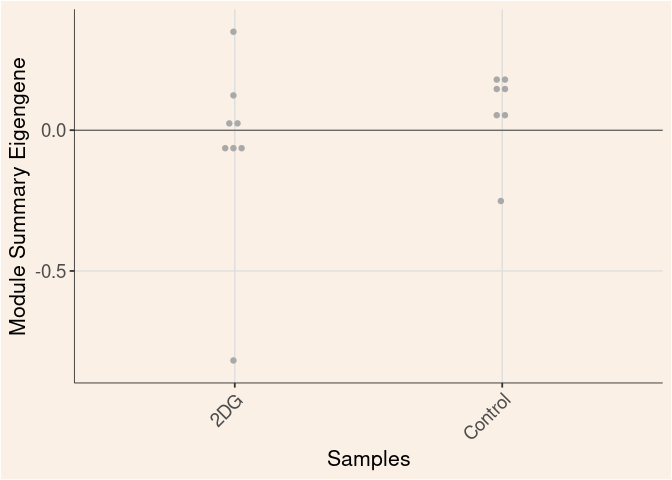
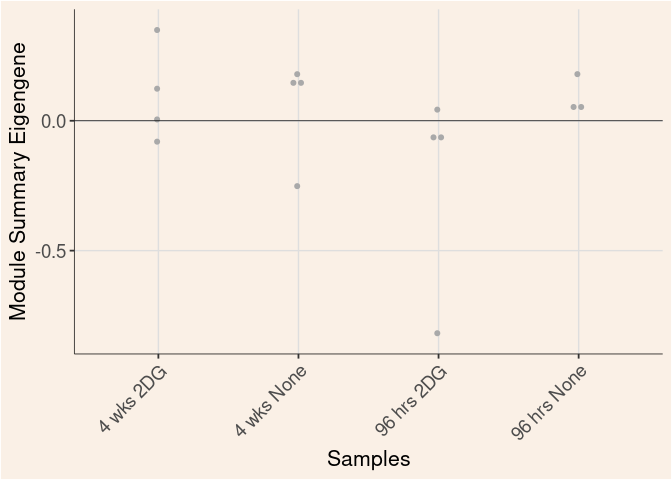
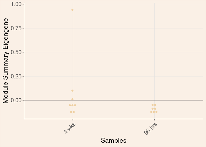
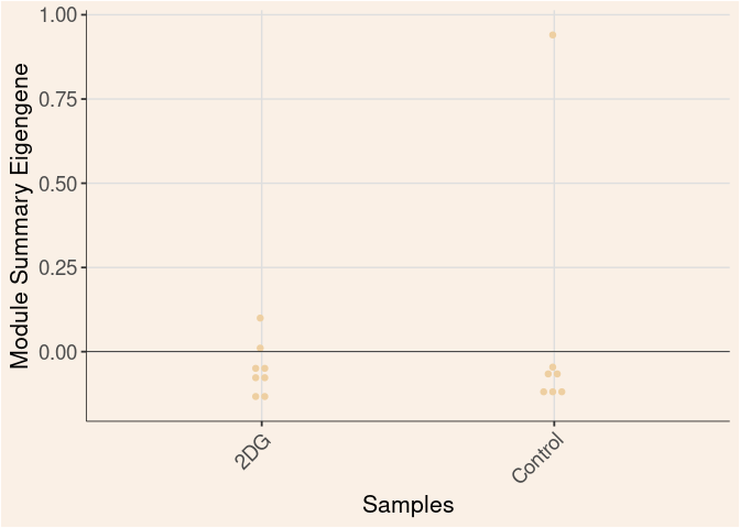
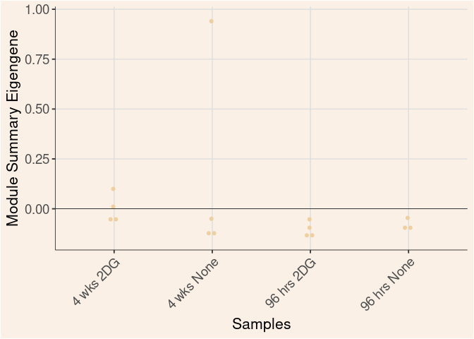
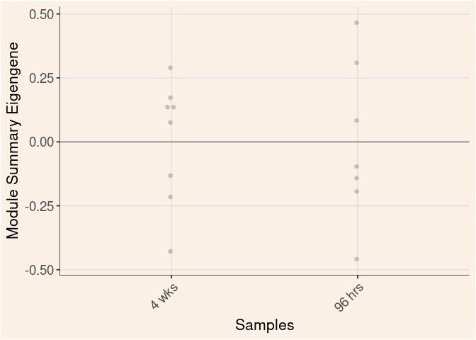
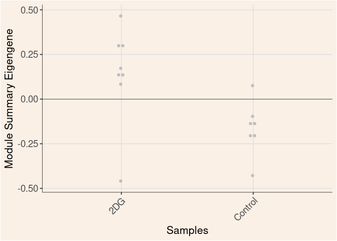
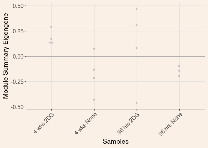
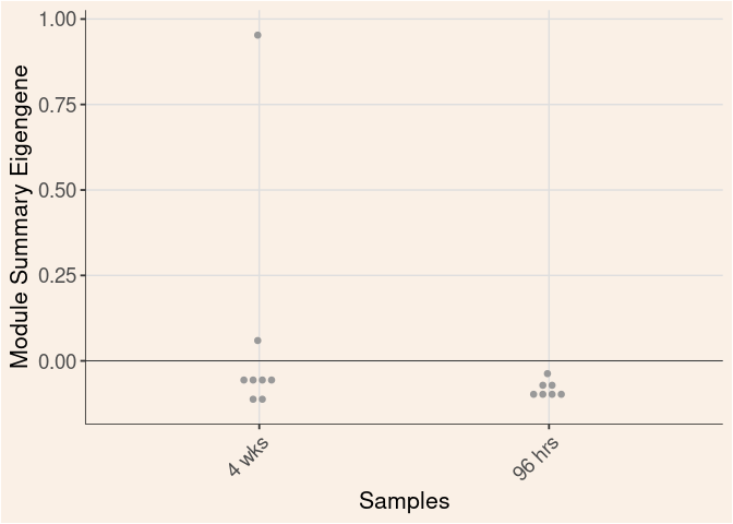
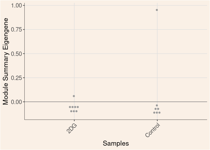
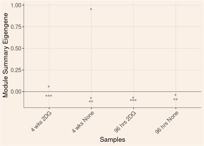
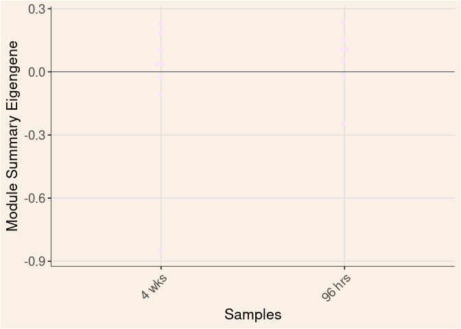
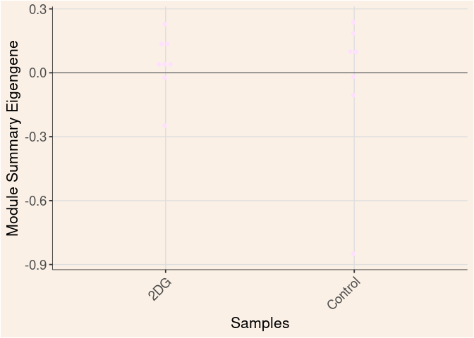
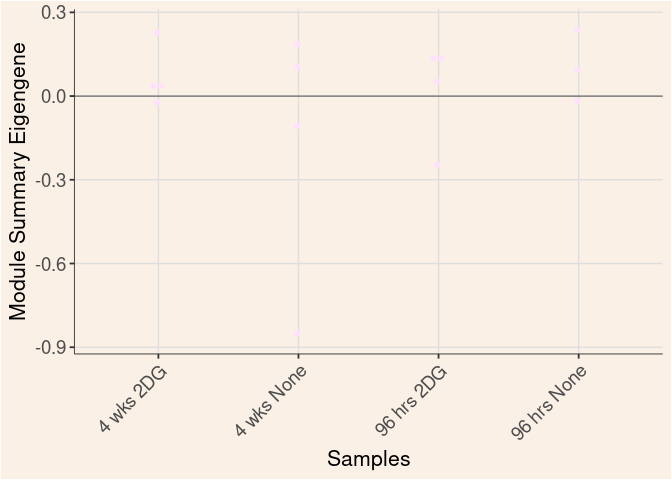
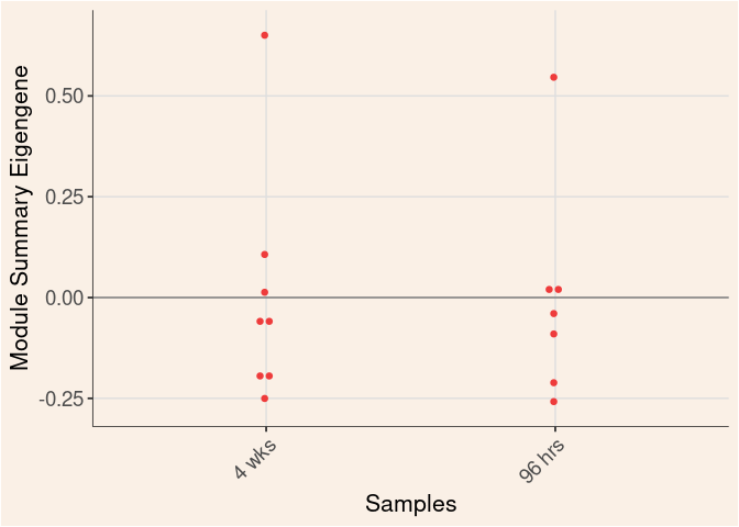
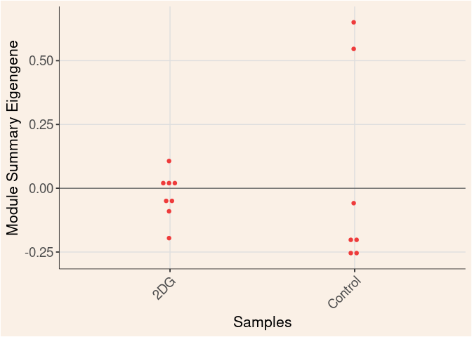
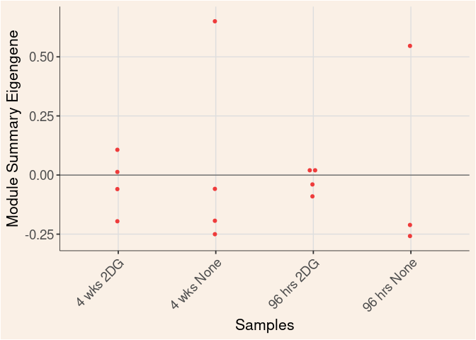
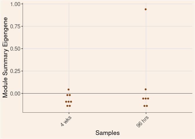
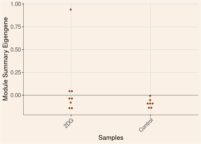
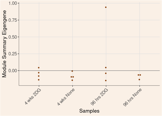
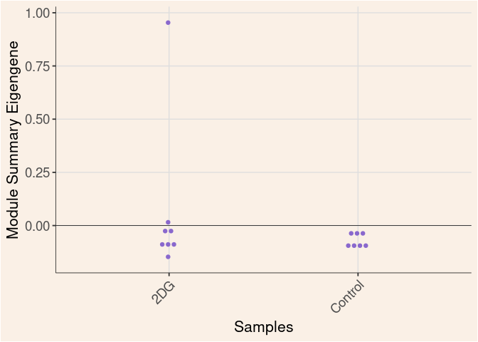
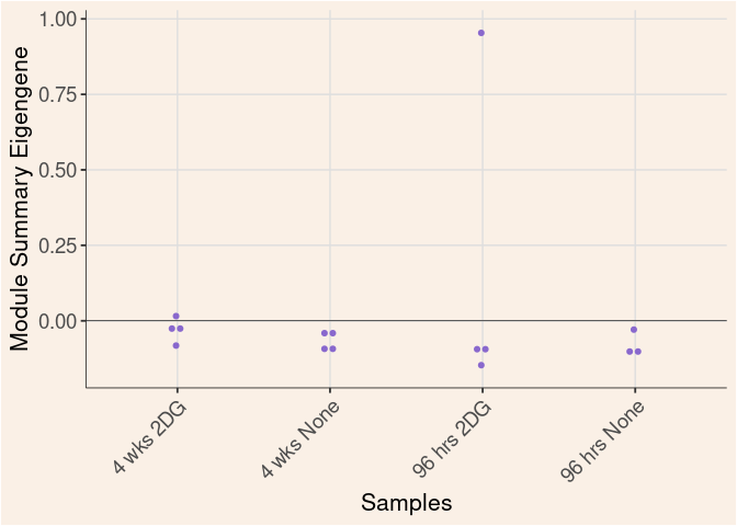
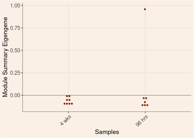
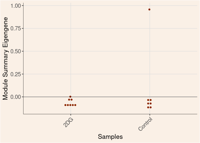
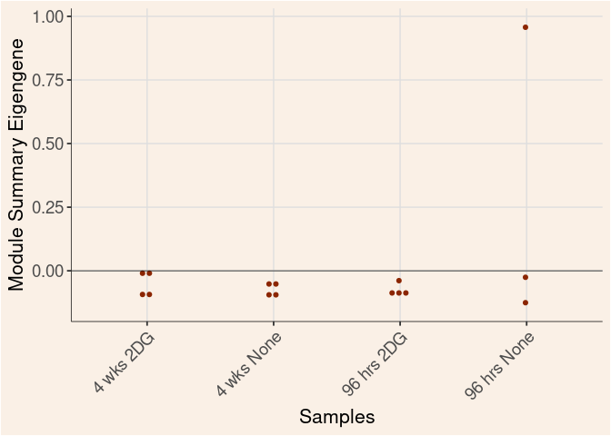
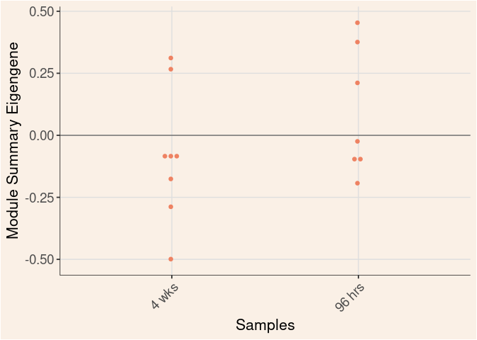
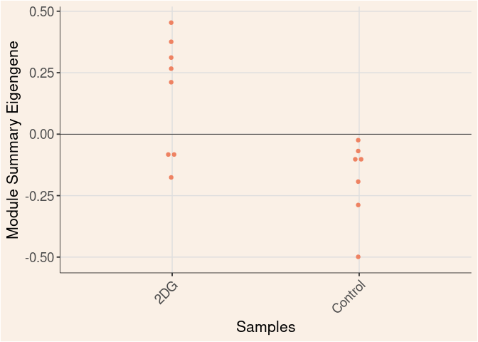
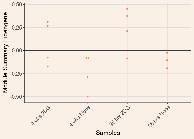
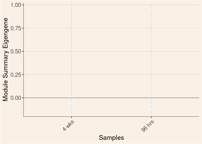
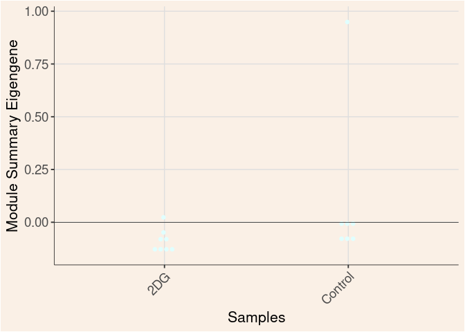
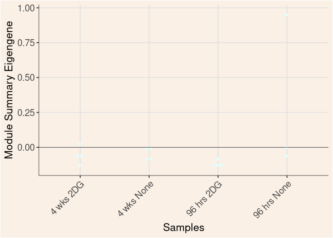
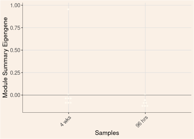
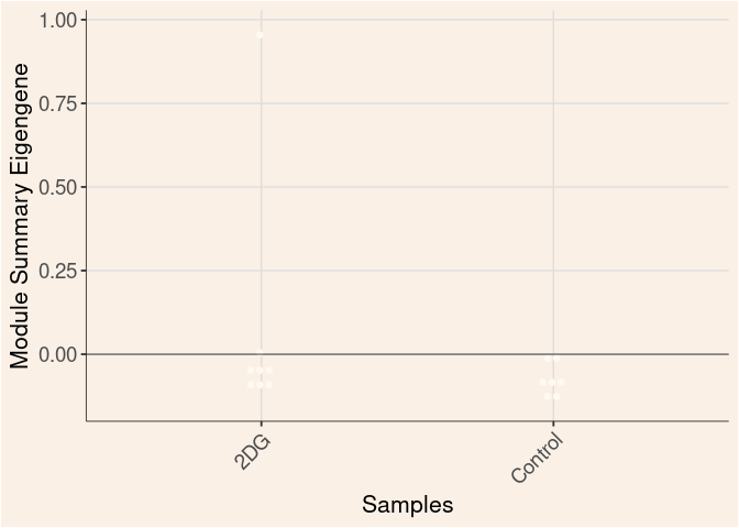
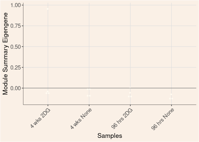
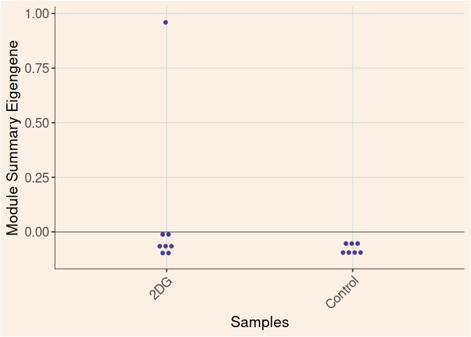
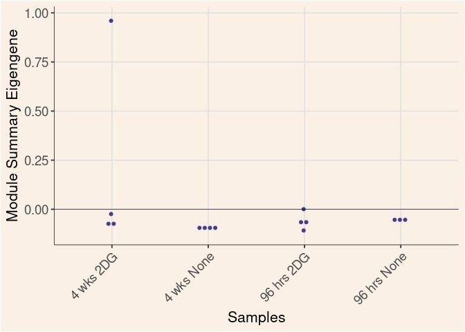
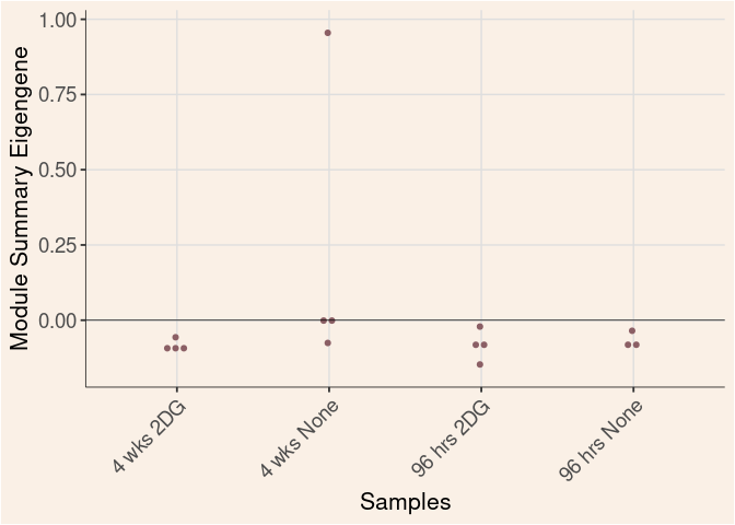
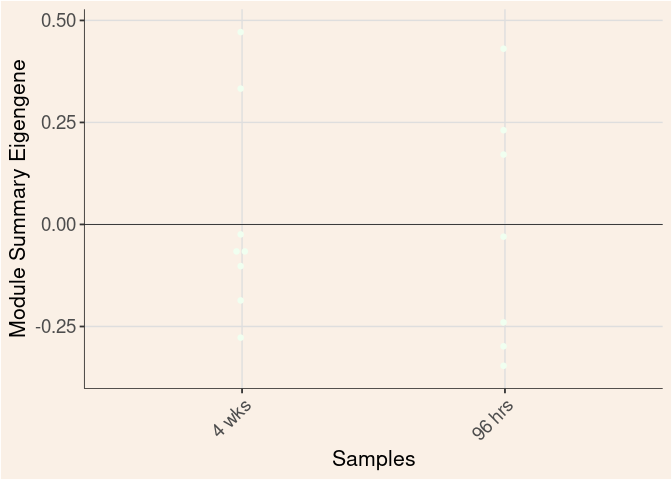
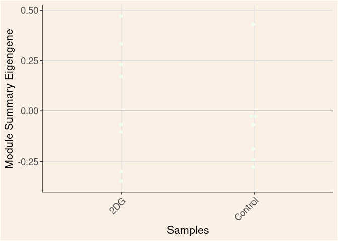
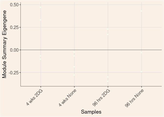
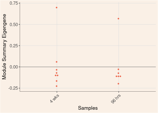
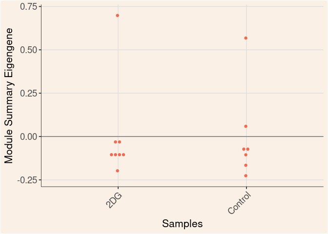
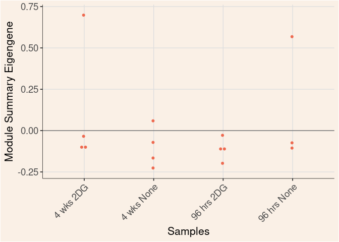
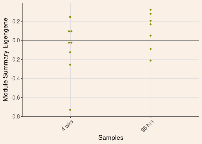
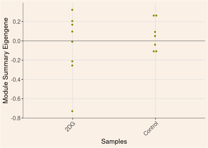
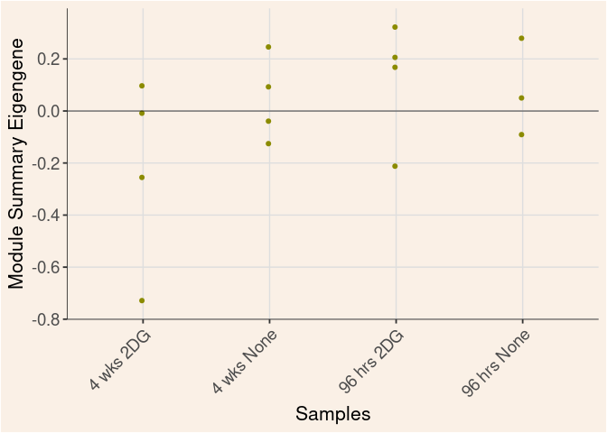
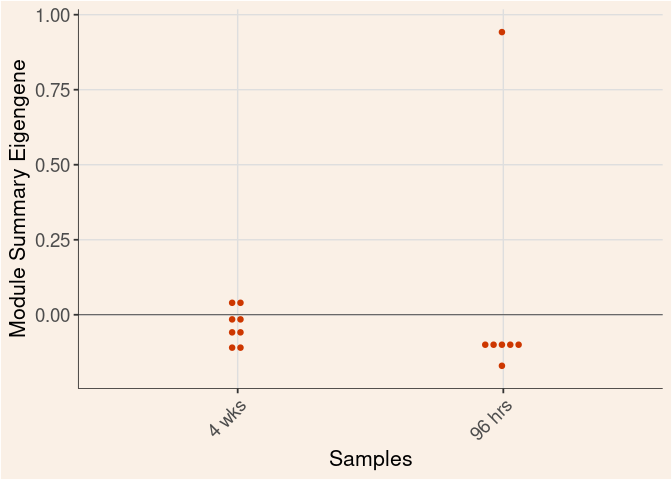
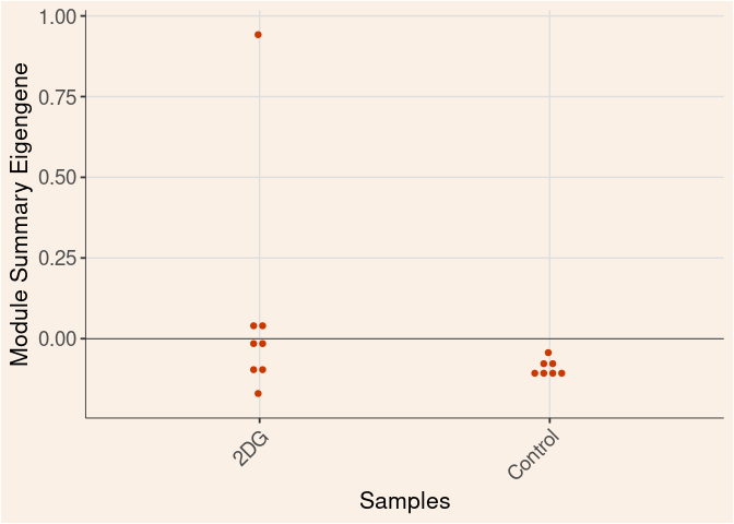
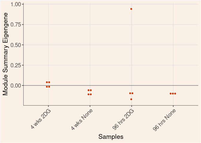
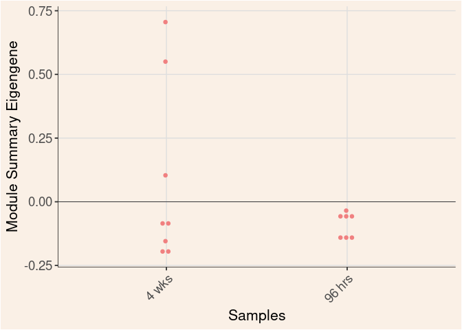
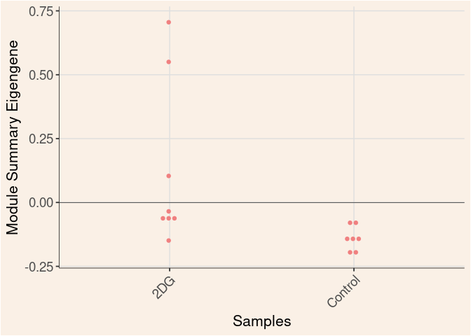
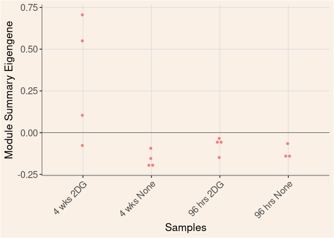
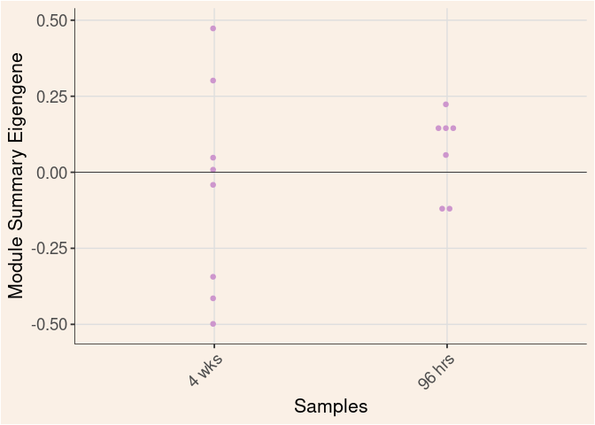
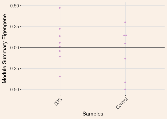
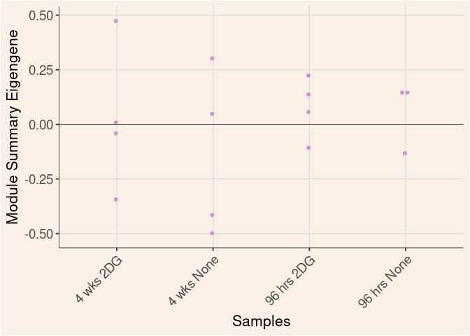
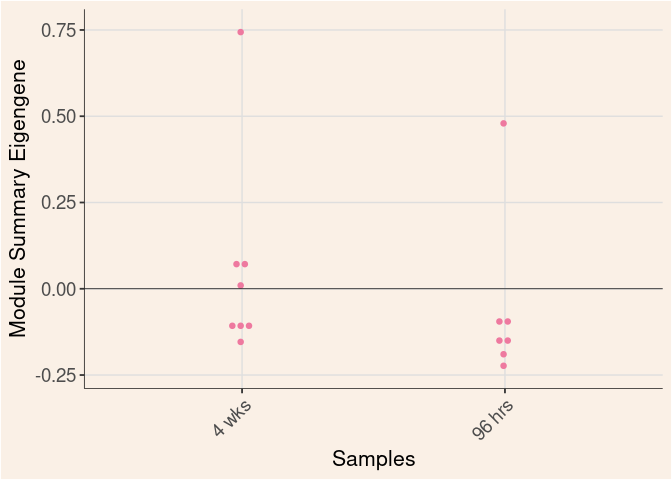
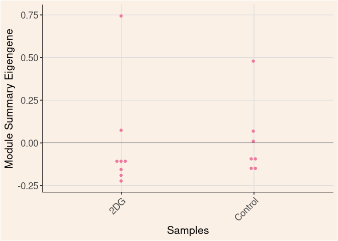
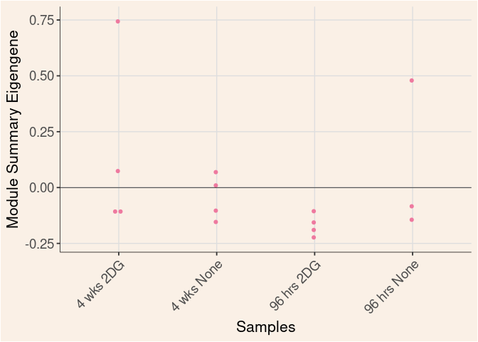
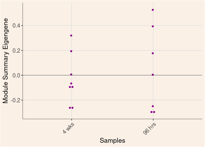
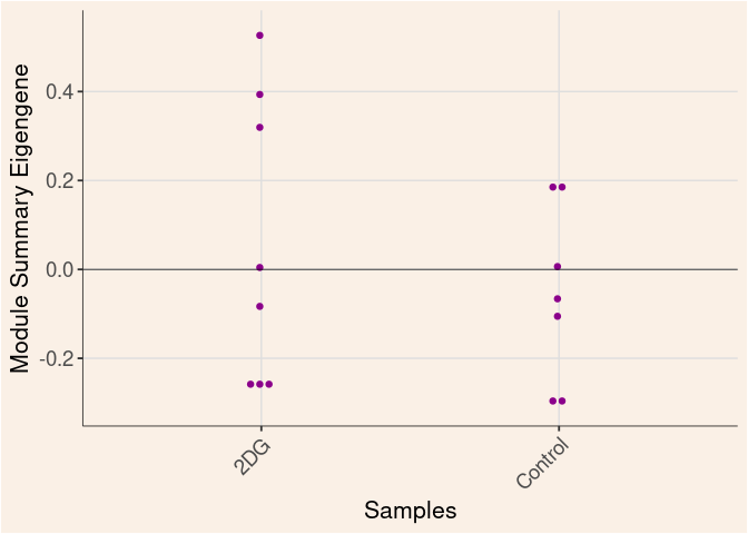
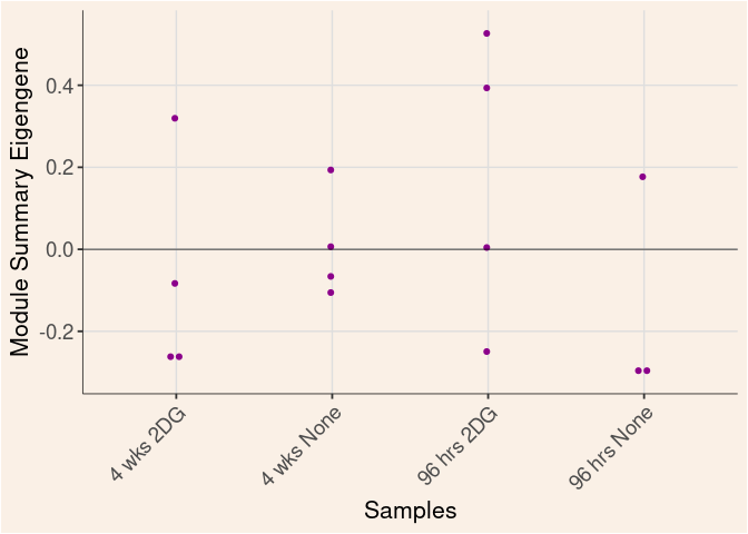
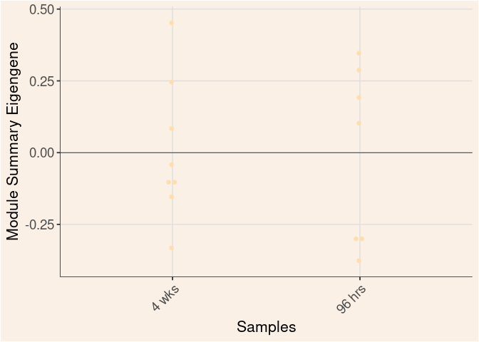
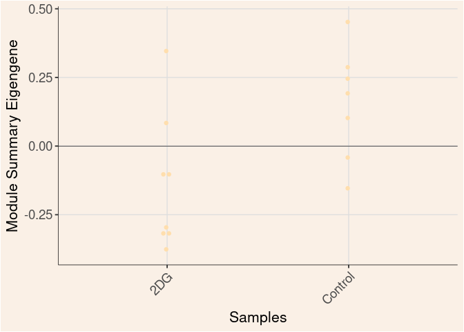
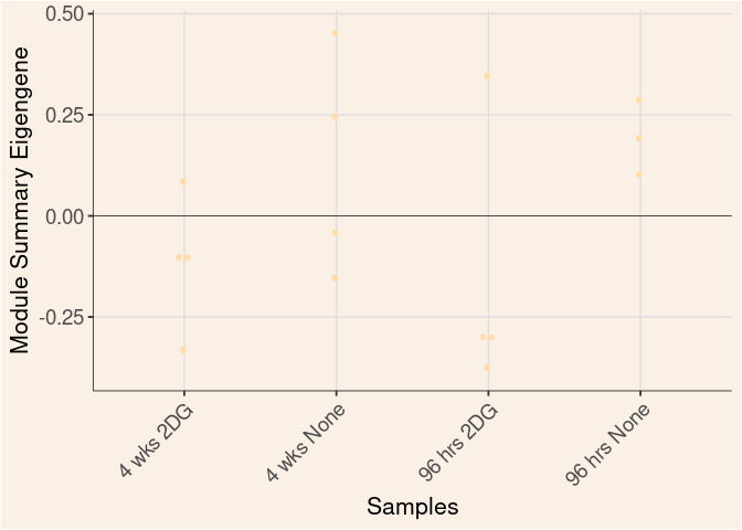
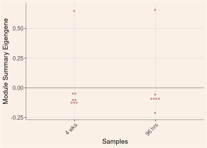
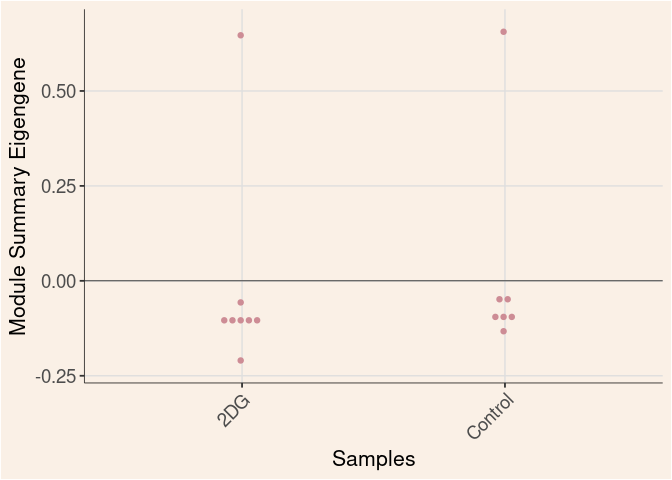
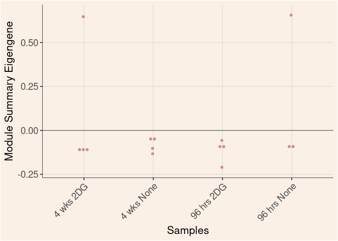
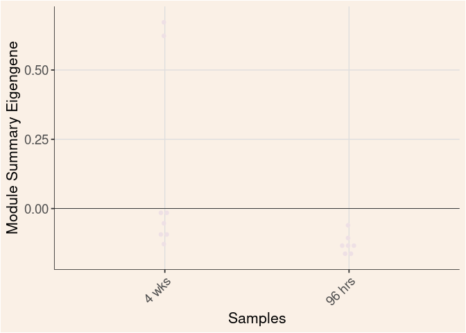
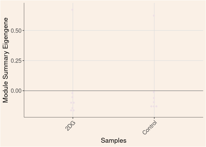
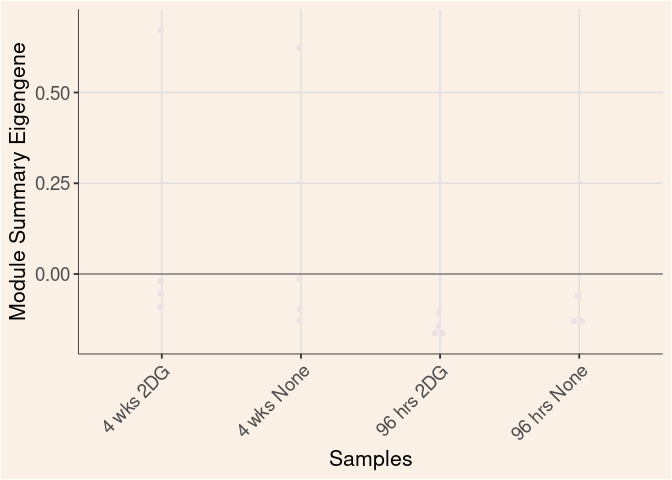
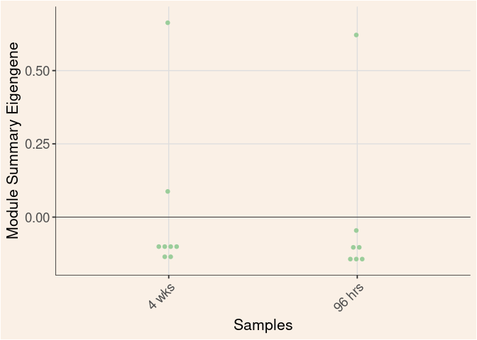
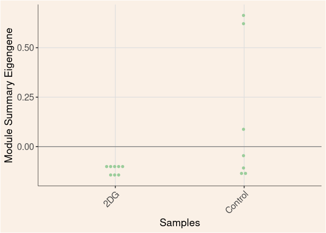
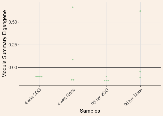
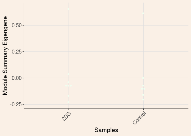
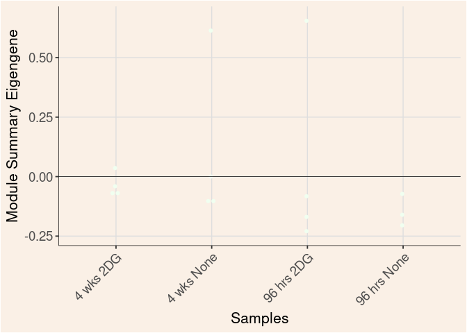
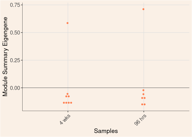
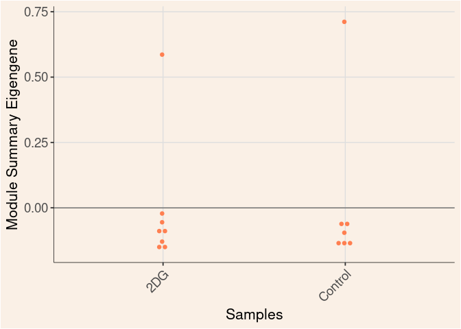
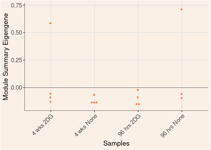
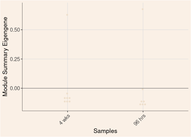
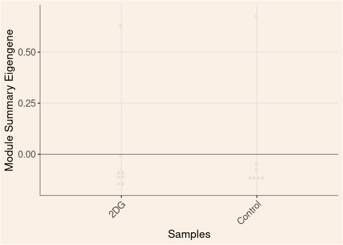
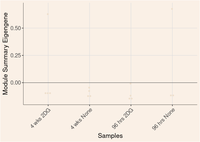
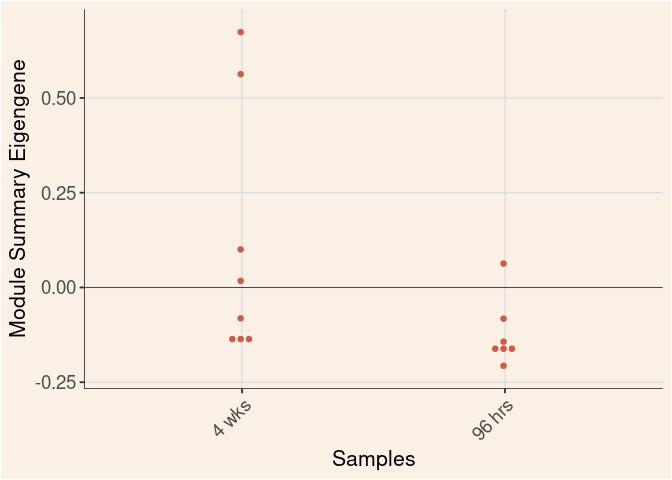
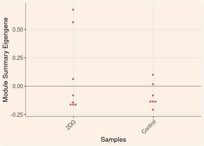
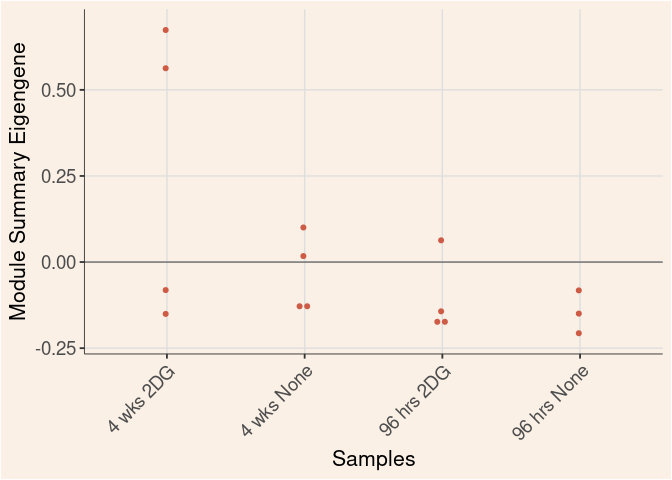
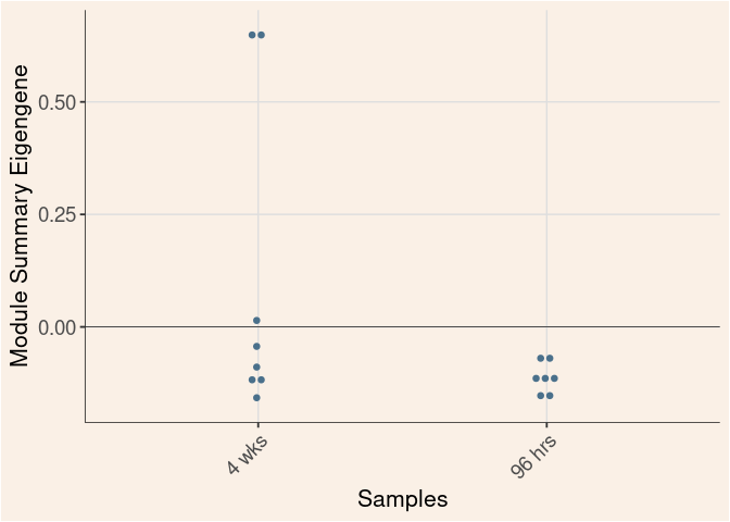
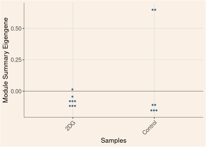
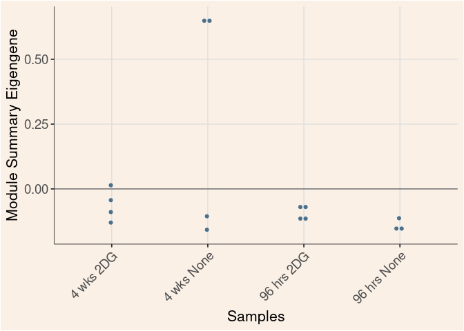
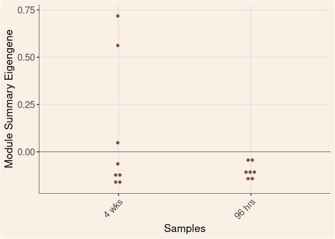
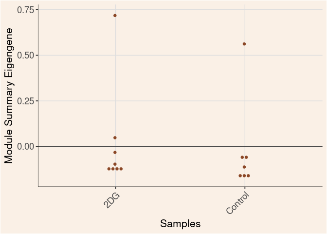
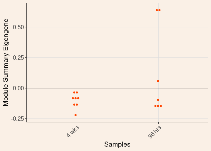
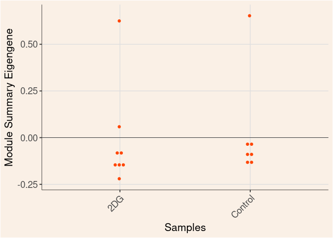
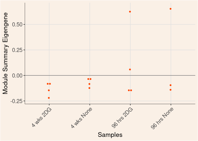
Module Sample Contribution Dot plot
dot.plot(eigens)brown4 Module
Time
Treatment
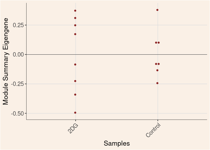
Time_by_Treatment
bisque4 Module
Time
Treatment
Time_by_Treatment
lightsteelblue1 Module
Time
Treatment
Time_by_Treatment
firebrick4 Module
Time
Treatment
Time_by_Treatment
turquoise Module
Time

Treatment
Time_by_Treatment
purple Module
Time
Treatment
Time_by_Treatment
green Module
Time
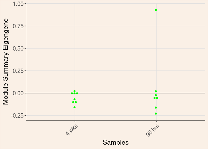
Treatment
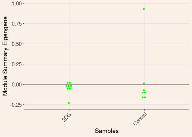
Time_by_Treatment
darkgrey Module
Time
Treatment
Time_by_Treatment
navajowhite2 Module
Time
Treatment
Time_by_Treatment
grey Module
Time
Treatment
Time_by_Treatment
grey60 Module
Time
Treatment
Time_by_Treatment
thistle1 Module
Time
Treatment
Time_by_Treatment
brown2 Module
Time
Treatment
Time_by_Treatment
saddlebrown Module
Time
Treatment
Time_by_Treatment
mediumpurple3 Module
Time

Treatment
Time_by_Treatment
orangered4 Module
Time
Treatment
Time_by_Treatment
salmon2 Module
Time
Treatment
Time_by_Treatment
lightcyan1 Module
Time
Treatment
Time_by_Treatment
floralwhite Module
Time
Treatment
Time_by_Treatment
darkslateblue Module
Time

Treatment
Time_by_Treatment
lightpink4 Module
Time

Treatment

Time_by_Treatment
honeydew1 Module
Time
Treatment
Time_by_Treatment
coral2 Module
Time
Treatment
Time_by_Treatment
yellow4 Module
Time
Treatment
Time_by_Treatment
orangered3 Module
Time
Treatment
Time_by_Treatment
lightcoral Module
Time
Treatment
Time_by_Treatment
plum3 Module
Time
Treatment
Time_by_Treatment
palevioletred2 Module
Time
Treatment
Time_by_Treatment
magenta4 Module
Time
Treatment
Time_by_Treatment
navajowhite1 Module
Time
Treatment
Time_by_Treatment
lightpink3 Module
Time
Treatment
Time_by_Treatment
lavenderblush2 Module
Time
Treatment
Time_by_Treatment
darkseagreen3 Module
Time
Treatment
Time_by_Treatment
honeydew Module
Time

Treatment
Time_by_Treatment
coral Module
Time
Treatment
Time_by_Treatment
antiquewhite2 Module
Time
Treatment
Time_by_Treatment
coral3 Module
Time
Treatment
Time_by_Treatment
skyblue4 Module
Time
Treatment
Time_by_Treatment
sienna4 Module
Time
Treatment
Time_by_Treatment

orangered1 Module
Time
Treatment
Time_by_Treatment
Analysis performed by Ann Wells
The Carter Lab The Jackson Laboratory 2023
ann.wells@jax.org