Introduction and Data files

This dataset contains nine tissues (heart, hippocampus, hypothalamus, kidney, liver, prefrontal cortex, skeletal muscle, small intestine, and spleen) from C57BL/6J mice that were fed 2-deoxyglucose (6g/L) through their drinking water for 96hrs or 4wks. 96hr mice were given their 2DG treatment 2 weeks after the other cohort started the 4 week treatment. The organs from the mice were harvested and processed for metabolomics and transcriptomics. The data in this document pertains to the transcriptomics data only. The counts that were used were FPKM normalized before being log transformed. It was determined that sample A113 had low RNAseq quality and through further analyses with PCA, MA plots, and clustering was an outlier and will be removed for the rest of the analyses performed. This document will determine the overall summary expression of each module across the main effects, as well as, assess the significance of each main effect and their interaction, using ANOVA, for each module and assess potential interactions visually for each module.

needed.packages <- c("tidyverse", "here", "functional", "gplots", "dplyr", "GeneOverlap", "R.utils", "reshape2","magrittr","data.table", "RColorBrewer","preprocessCore", "ARTool","emmeans", "phia", "gProfileR", "WGCNA","plotly", "pheatmap","pander", "kableExtra")
for(i in 1:length(needed.packages)){library(needed.packages[i], character.only = TRUE)}

source(here("source_files","WGCNA_source.R"))
source(here("source_files","plot_theme.R"))

tdata.FPKM.sample.info <- readRDS(here("Data","20190406_RNAseq_B6_4wk_2DG_counts_phenotypes.RData"))

tdata.FPKM <- readRDS(here("Data","20190406_RNAseq_B6_4wk_2DG_counts_numeric.RData"))

log.tdata.FPKM <- log(tdata.FPKM + 1)
log.tdata.FPKM <- as.data.frame(log.tdata.FPKM)

log.tdata.FPKM.sample.info <- cbind(log.tdata.FPKM, tdata.FPKM.sample.info[,27238:27240])

log.tdata.FPKM.sample.info <- log.tdata.FPKM.sample.info %>% rownames_to_column() %>% filter(rowname != "A113") %>% column_to_rownames()

log.tdata.FPKM.subset <- log.tdata.FPKM[,colMeans(log.tdata.FPKM != 0) > 0.5] 

log.tdata.FPKM.sample.info.subset <- cbind(log.tdata.FPKM.subset,tdata.FPKM.sample.info[,27238:27240])
log.tdata.FPKM.sample.info.subset <- log.tdata.FPKM.sample.info.subset %>% rownames_to_column() %>% filter(rowname != "A113") %>% column_to_rownames()

log.tdata.FPKM.sample.info.subset.small.intestine <- log.tdata.FPKM.sample.info.subset %>% rownames_to_column() %>% filter(Tissue == "Small Intestine") %>% column_to_rownames()

log.tdata.FPKM.sample.info.subset.small.intestine$Treatment[log.tdata.FPKM.sample.info.subset.small.intestine$Treatment=="None"] <- "Control"

log.tdata.FPKM.sample.info.subset.small.intestine <- cbind(log.tdata.FPKM.sample.info.subset.small.intestine, Time.Treatment = paste(log.tdata.FPKM.sample.info.subset.small.intestine$Time, log.tdata.FPKM.sample.info.subset.small.intestine$Treatment))

module.labels <- readRDS(here("Data","Small Intestine","log.tdata.FPKM.sample.info.subset.small.intestine.WGCNA.module.labels.RData"))
module.eigens <- readRDS(here("Data","Small Intestine","log.tdata.FPKM.sample.info.subset.small.intestine.WGCNA.module.eigens.RData"))
modules <- readRDS(here("Data","Small Intestine","log.tdata.FPKM.sample.info.subset.small.intestine.WGCNA.module.membership.RData"))
net.deg <- readRDS(here("Data","Small Intestine","Chang_2DG_BL6_connectivity_small_intestine.RData"))
ensembl.location <- readRDS(here("Data","Ensembl_gene_id_and_location.RData"))

Eigengene Stratification

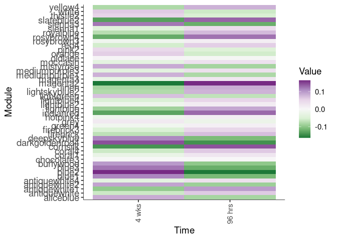
Eigengene were stratified by time and treatment. The heatmap is a matrix of the average eigengene value for each level of the trait.

factors <- c("Time","Treatment","Time.Treatment")
eigenmetabolite(factors,log.tdata.FPKM.sample.info.subset.small.intestine)

Time

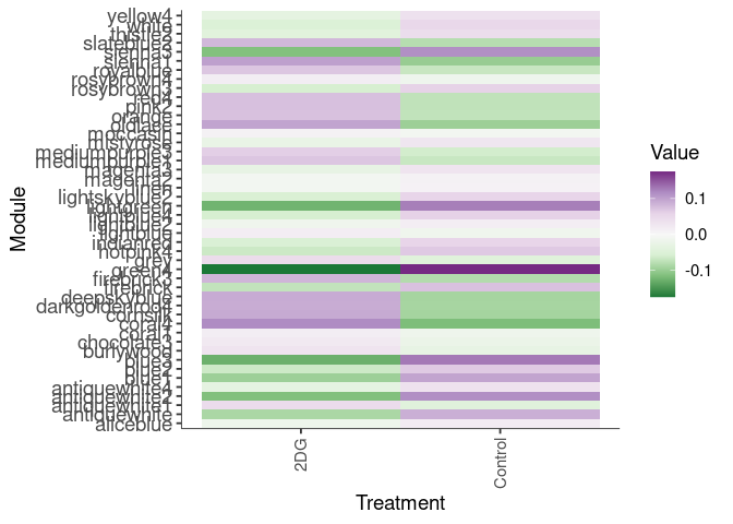
Treatment

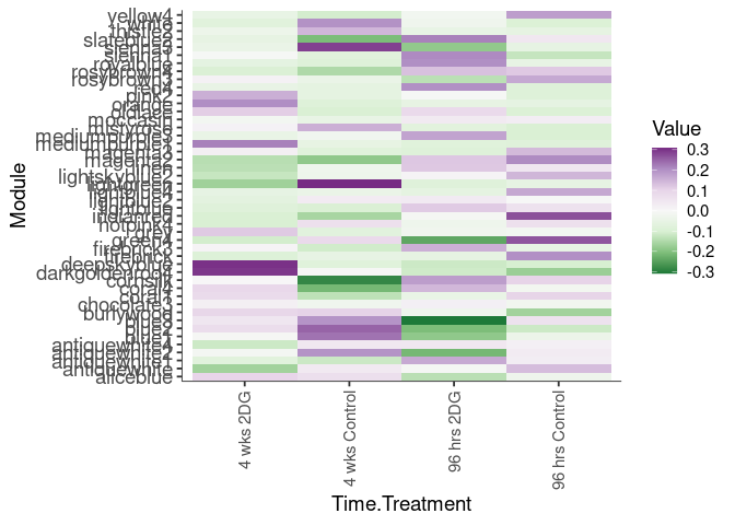
Time.Treatment

ANOVA

An ANOVA using aligned rank transformation was performed for each module. The full model is y ~ time + treatment + time:treatment.

# Three-Way ANOVA for each Eigenmetabolite
model.data = dplyr::bind_cols(module.eigens[rownames(log.tdata.FPKM.sample.info.subset.small.intestine),], log.tdata.FPKM.sample.info.subset.small.intestine[,c("Time","Treatment")])
model.data$Time <- as.factor(model.data$Time)
model.data$Treatment <- as.factor(model.data$Treatment)

final.anova <- list()
for (m in colnames(module.eigens)) {
  a <- art(data = model.data, model.data[,m] ~ Time*Treatment)
  model <- anova(a)
  adjust <- p.adjust(model$`Pr(>F)`, method = "BH")
  
  final.anova[[m]] <- cbind(model, adjust)
}

Cornsilk Module

DT.table(final.anova[[1]])

Blue1 Module

DT.table(final.anova[[2]])

Rosybrown3 Module

DT.table(final.anova[[3]])

Antiquewhite2 Module

DT.table(final.anova[[4]])

Aliceblue Module

DT.table(final.anova[[5]])

Blue3 Module

DT.table(final.anova[[6]])

Coral1 Module

DT.table(final.anova[[7]])

Magenta3 Module

DT.table(final.anova[[8]])

Burlywood Module

DT.table(final.anova[[9]])

Lightblue2 Module

DT.table(final.anova[[10]])

Green4 Module

DT.table(final.anova[[11]])

Antiquewhite1 Module

DT.table(final.anova[[12]])

Sienna3 Module

DT.table(final.anova[[13]])

Coral4 Module

DT.table(final.anova[[14]])

Blue2 Module

DT.table(final.anova[[15]])

Antiquewhite4 Module

DT.table(final.anova[[16]])

Firebrick Module

DT.table(final.anova[[17]])

Deepskyblue Module

DT.table(final.anova[[18]])

Hotpink4 Module

DT.table(final.anova[[19]])

Grey Module

DT.table(final.anova[[20]])

Lightgreen Module

DT.table(final.anova[[21]])

Rosybrown4 Module

DT.table(final.anova[[22]])

Royalblue Module

DT.table(final.anova[[23]])

Orange Module

DT.table(final.anova[[24]])

White Module

DT.table(final.anova[[25]])

Slateblue2 Module

DT.table(final.anova[[26]])

Magenta2 Module

DT.table(final.anova[[27]])

Mediumpurple3 Module

DT.table(final.anova[[28]])

Thistle2 Module

DT.table(final.anova[[29]])

Yellow4 Module

DT.table(final.anova[[30]])

Indianred Module

DT.table(final.anova[[31]])

Antiquewhite Module

DT.table(final.anova[[32]])

Mediumpurple1 Module

DT.table(final.anova[[33]])

Lightblue4 Module

DT.table(final.anova[[34]])

Firebrick3 Module

DT.table(final.anova[[35]])

Mistyrose Module

DT.table(final.anova[[36]])

Moccasin Module

DT.table(final.anova[[37]])

Chocolate3 Module

DT.table(final.anova[[38]])

Pink2 Module

DT.table(final.anova[[39]])

Sienna1 Module

DT.table(final.anova[[40]])

Darkgoldenrod4 Module

DT.table(final.anova[[41]])

Lightskyblue2 Module

DT.table(final.anova[[42]])

Linen Module

DT.table(final.anova[[43]])

Oldlace Module

DT.table(final.anova[[44]])

Lightblue Module

DT.table(final.anova[[45]])

Red4 Module

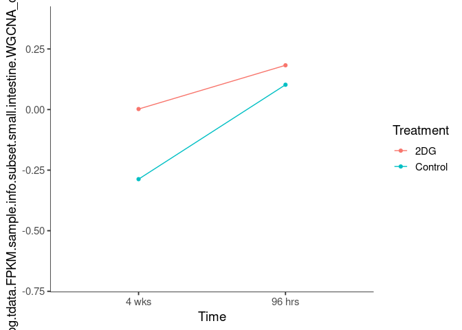
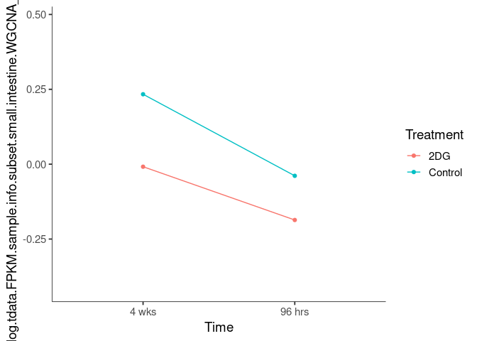
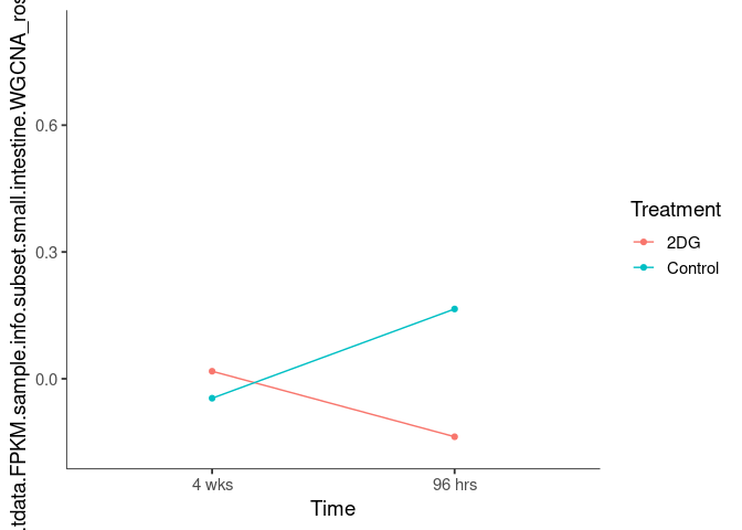
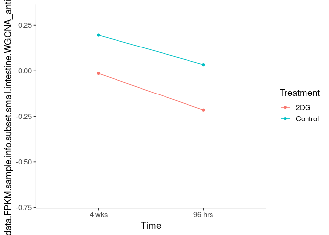
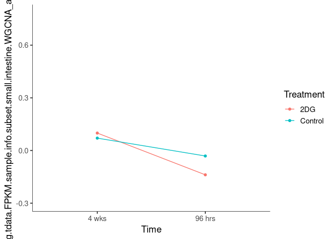
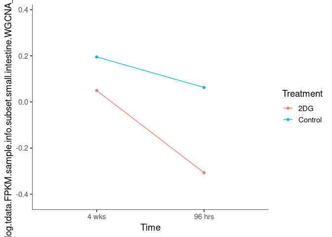
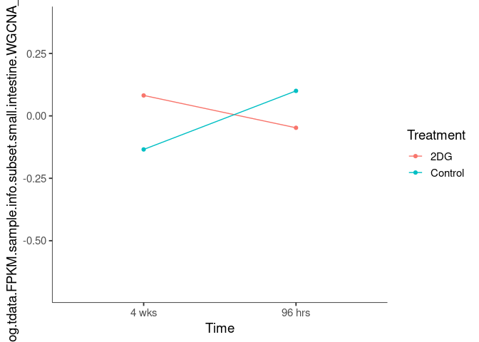
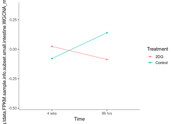
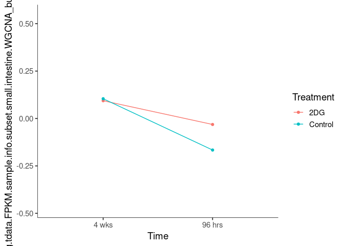
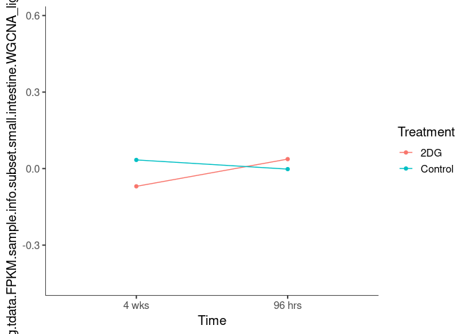
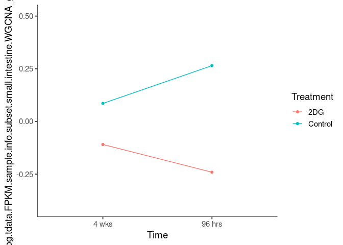
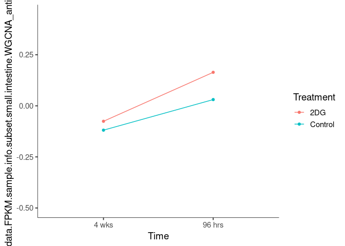
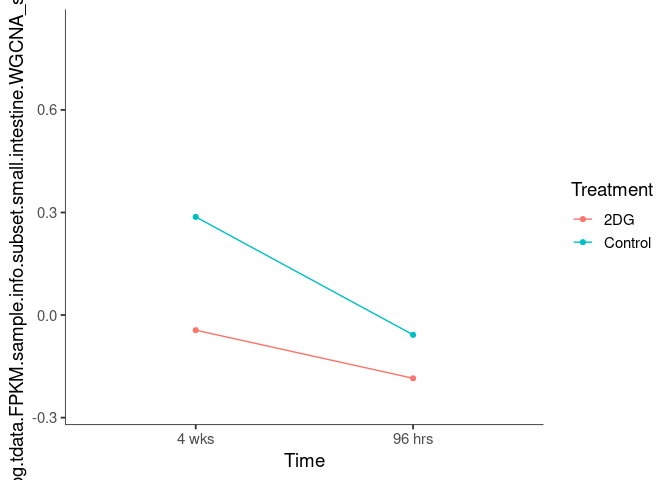
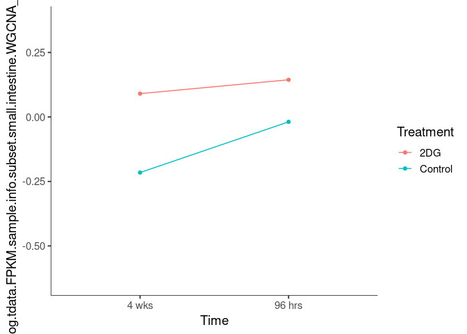
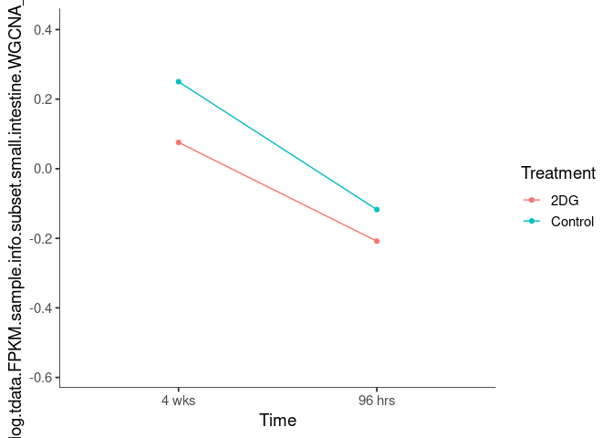
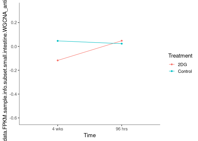
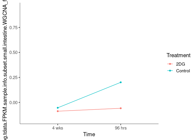
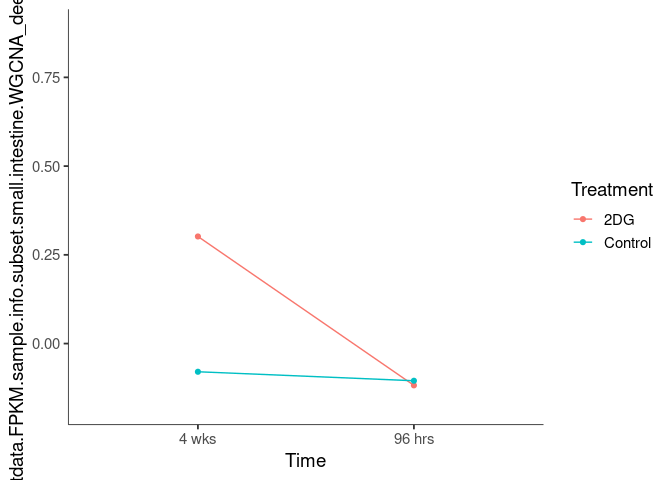
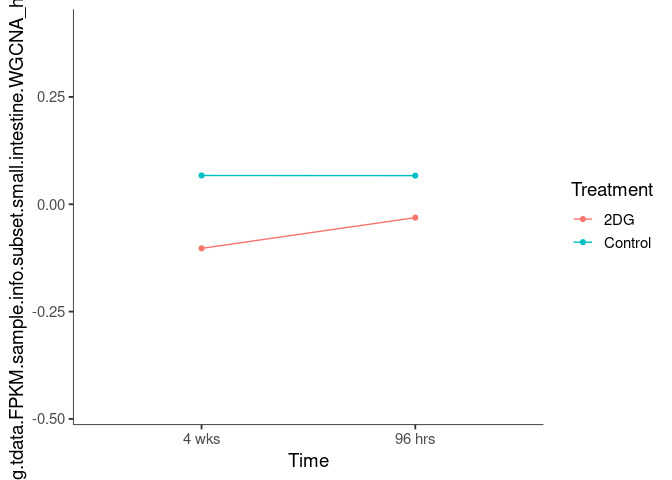
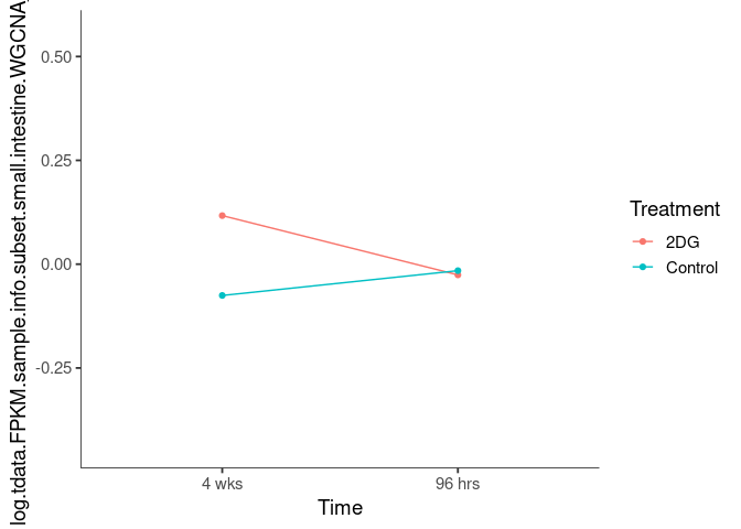
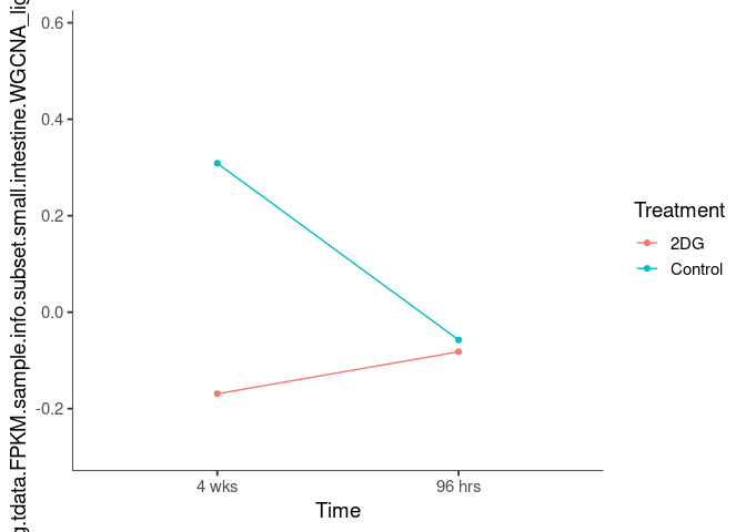
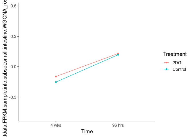
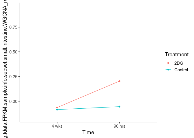
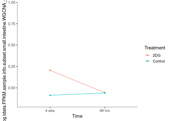
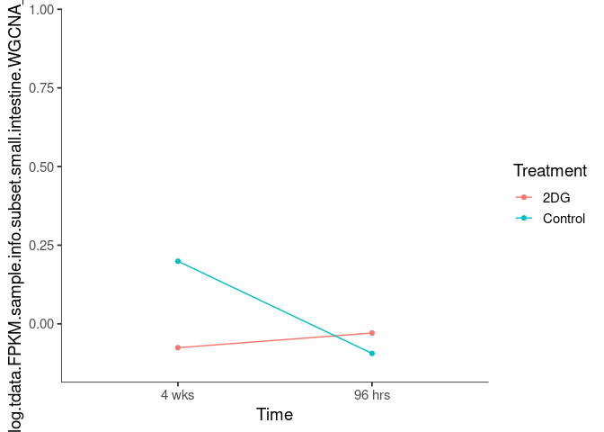
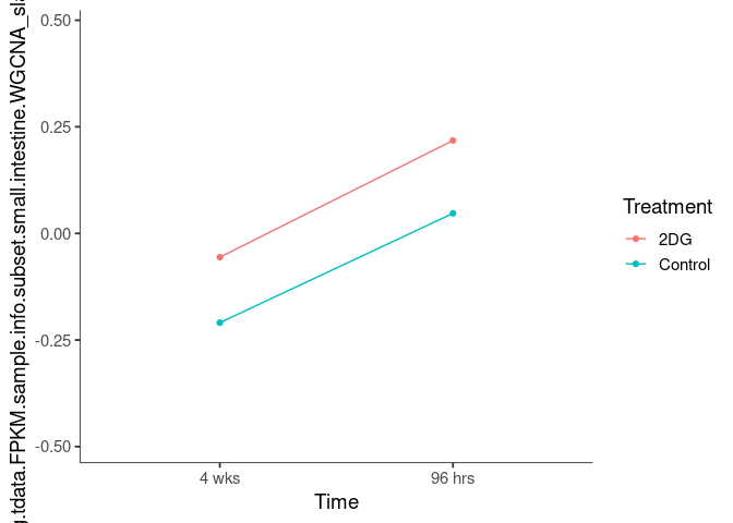
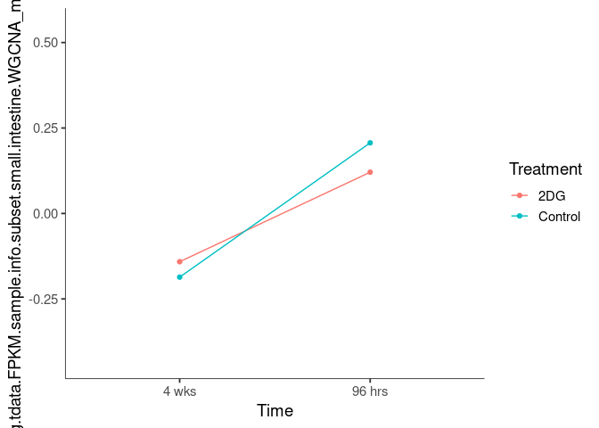
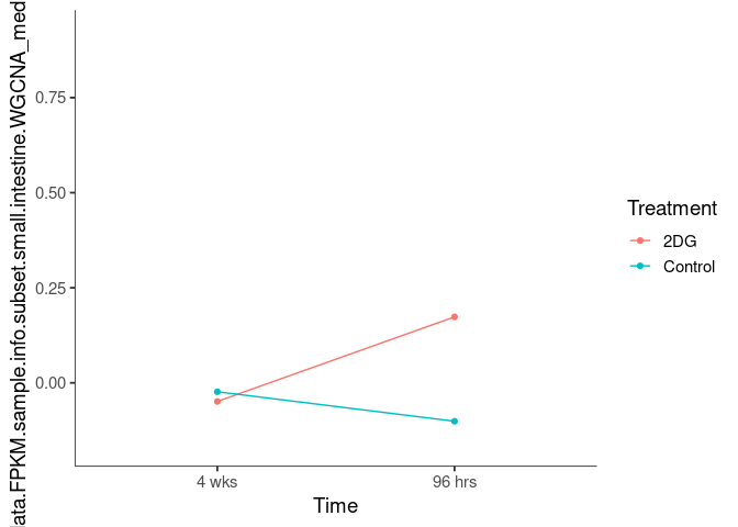
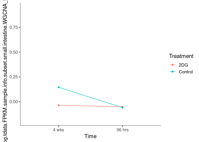
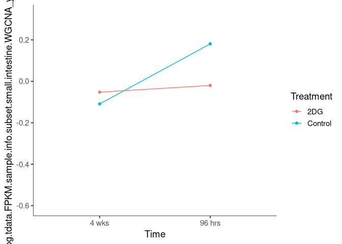
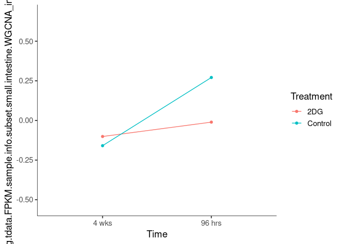
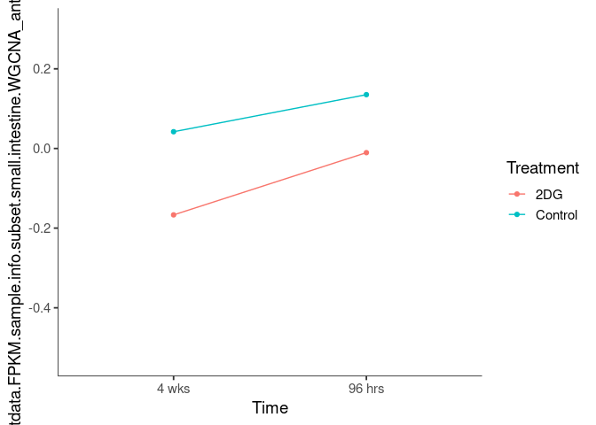
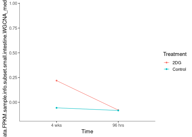
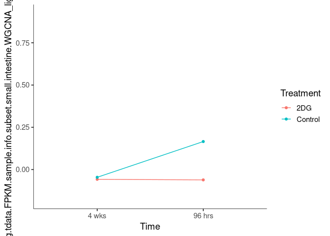
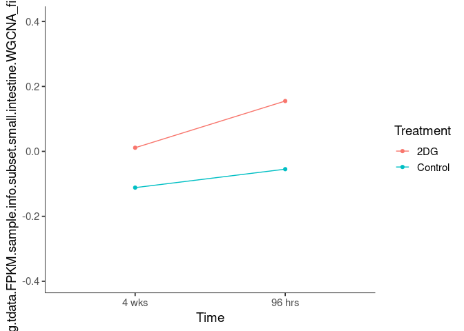
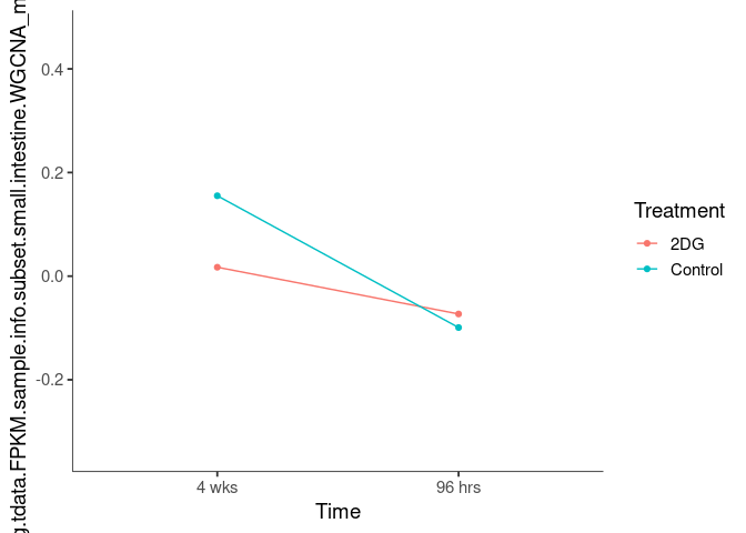
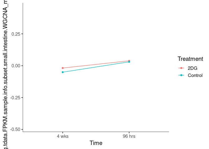
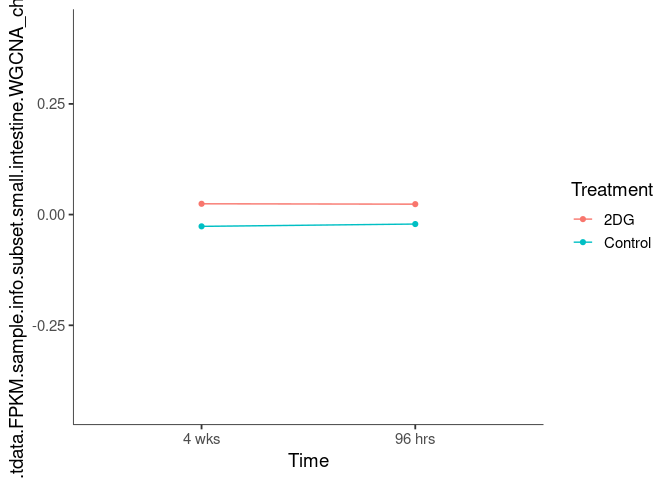
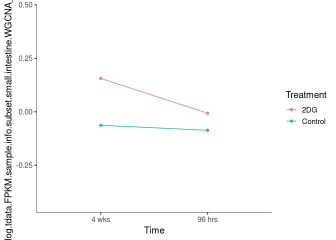
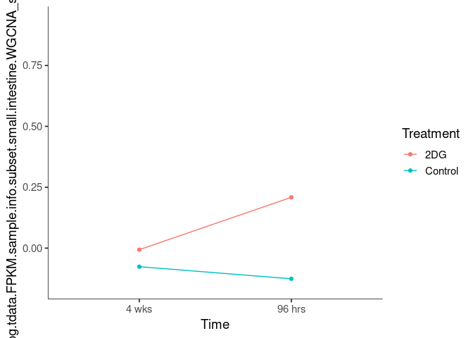
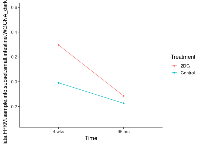
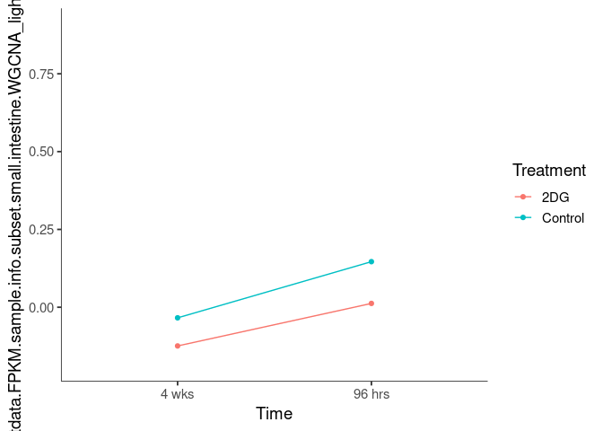
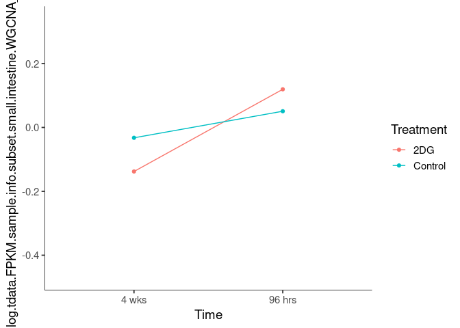
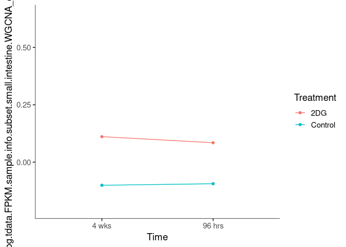
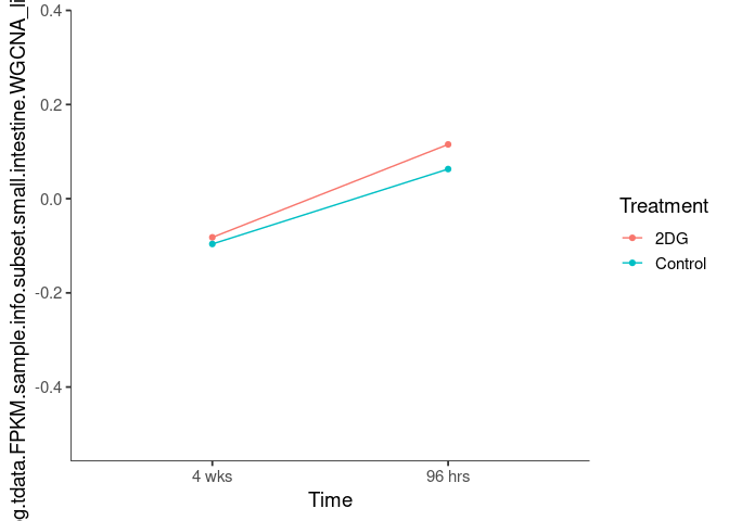
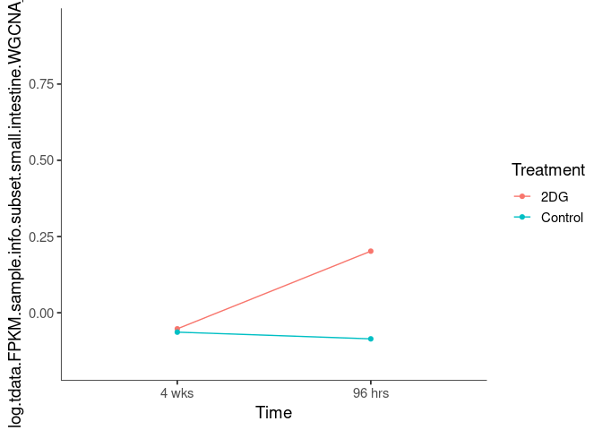
DT.table(final.anova[[46]])

Interaction plots

Interaction plots were created to identify which modules have a potential interaction between time and treatment. A potential interaction is identified when the two lines cross.

for (m in module.labels) {
  p = plot.interaction(model.data, "Time", "Treatment", resp = m)
  name <- sapply(str_split(m,"_"),"[",2)
  cat("\n###",name,"\n")
  print(p)
  cat("\n \n")
}